
Percentiles are a foundational tool for reasoning about system performance. They tell you not just what’s typical, but what your tail users are actually experiencing — and at scale, your tail users are the ones who churn, file support tickets, and define your reliability reputation.
This document covers not just what percentiles are, but how they’re computed, where they mislead you, and how to design systems around them.
What Is a Percentile?
A percentile represents the value below which a given percentage of observations fall.
If your p99 latency is 500ms, it means 99% of requests completed in under 500ms — and 1% took longer. At 10,000 requests per minute, that’s 100 users per minute experiencing degraded service.
The Distribution at a Glance
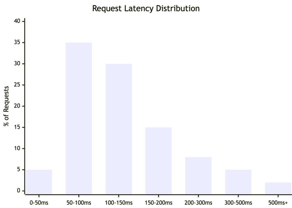
Most requests cluster at the fast end — but the right tail extends further than averages ever reveal. This shape is typical of production systems: fast for most, painful for some.
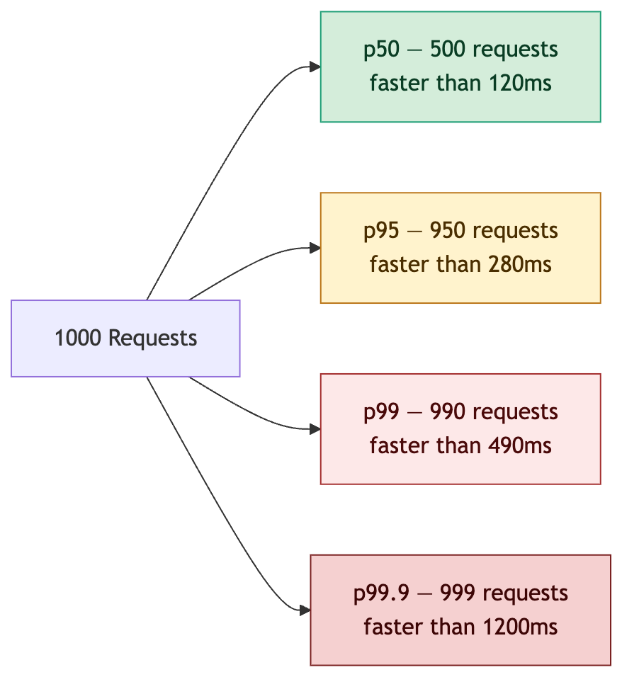
How Each Percentile Maps to Users
Why Averages Lie
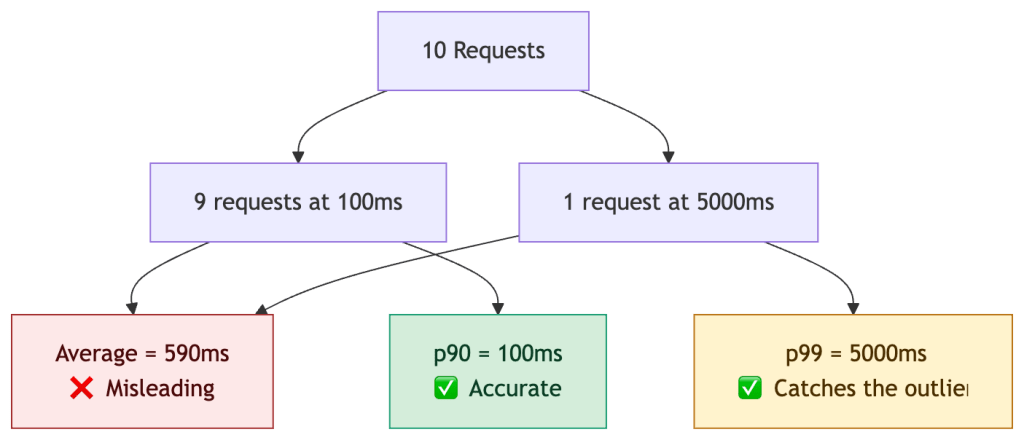
One slow request drags the average up significantly. Percentiles isolate outliers statistically, but do not explain causality. This is why average latency dashboards create misleading confidence about the real user experience.
Real-World Example: An E-Commerce Checkout
You’re running an online store capturing latency for 10,000 checkout requests per hour. Traffic spikes between 7–9pm. Your DB has a connection pool of 50.
| Percentile | Latency | What It Means |
|---|---|---|
| p50 | 95ms | Typical checkout feels instant |
| p75 | 180ms | Most users unaffected |
| p95 | 420ms | 500 users/hr experiencing noticeable lag |
| p99 | 1,100ms | 100 users/hr waiting over 1 second — frustrating |
| p99.9 | 4,800ms | ~10 users/hr at risk of cart abandonment |
Root cause of the p99 spike: The 1.1s tail correlates with cache miss bursts during traffic ramp-up and DB connection pool exhaustion under peak load. The average (130ms) looked healthy throughout.
The fix required three changes:
- Cache warming before peak traffic windows
- Query optimization to reduce connection hold time
- Connection pool tuning to shed load rather than queue
This is the key lesson: p99 tells you where to look; tracing tells you why.
How Percentiles Are Computed in Practice
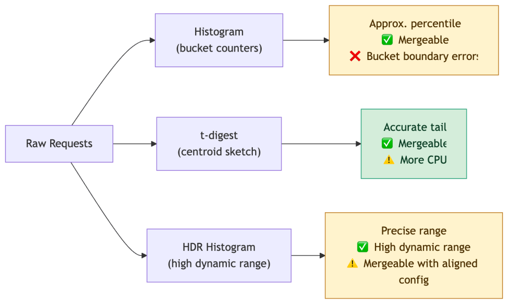
You rarely compute exact percentiles in production — the memory cost is prohibitive at scale. Real systems use approximations:
| Method | Used In | Accuracy | Tradeoff |
|---|---|---|---|
| Histograms | Prometheus | Moderate | Fixed buckets, fast, mergeable across instances |
| t-digest | Datadog, OpenTelemetry | High at tails | More compute, better p99/p99.9 accuracy |
| HDR Histogram | JVM systems, wrk | Very high | High dynamic range, larger memory footprint; mergeable but requires aligned bucket configuration |
| Summaries | Prometheus (legacy) | Exact | Cannot be aggregated across instances |
Note on cost: High-resolution histograms and tail-accurate sketches increase metrics cardinality, storage, and CPU usage — percentile accuracy is not free. Choose your method based on the criticality of the path being measured.
Critical: Prometheus summaries compute percentiles client-side and cannot be aggregated. If you sum p99s from two replicas, you get a meaningless number. Use histograms with
histogram_quantile()instead.
When Percentiles Mislead You
Percentiles are only as good as your data collection strategy. Three failure modes matter most in production.
1. Coordinated Omission
If your system slows down and stops accepting new requests, your measurement tool stops recording during the slowdown. The result: tail latency is systematically underreported.
A load test that sends 100 RPS but pauses on backpressure will miss the latency experienced during the pause. Tools like
wrk2use a coordinated omission correction; most others do not.
2. Low-Volume Distortion
p99 over 100 requests means only 1 data point defines your tail. That single request could be a fluke — a GC pause, a cold start, a network blip. It’s statistically meaningless.
Rule of thumb: You need at least 1,000 samples for p99 to be stable, and 10,000+ for p99.9. Below these thresholds, widen your time window or report p95 instead.
3. Sampling Bias
If you drop traces or logs under load (a common cost-saving measure), you’re more likely to drop fast requests than slow ones — slow requests hold resources longer and are more likely to be captured. This inflates apparent percentiles.
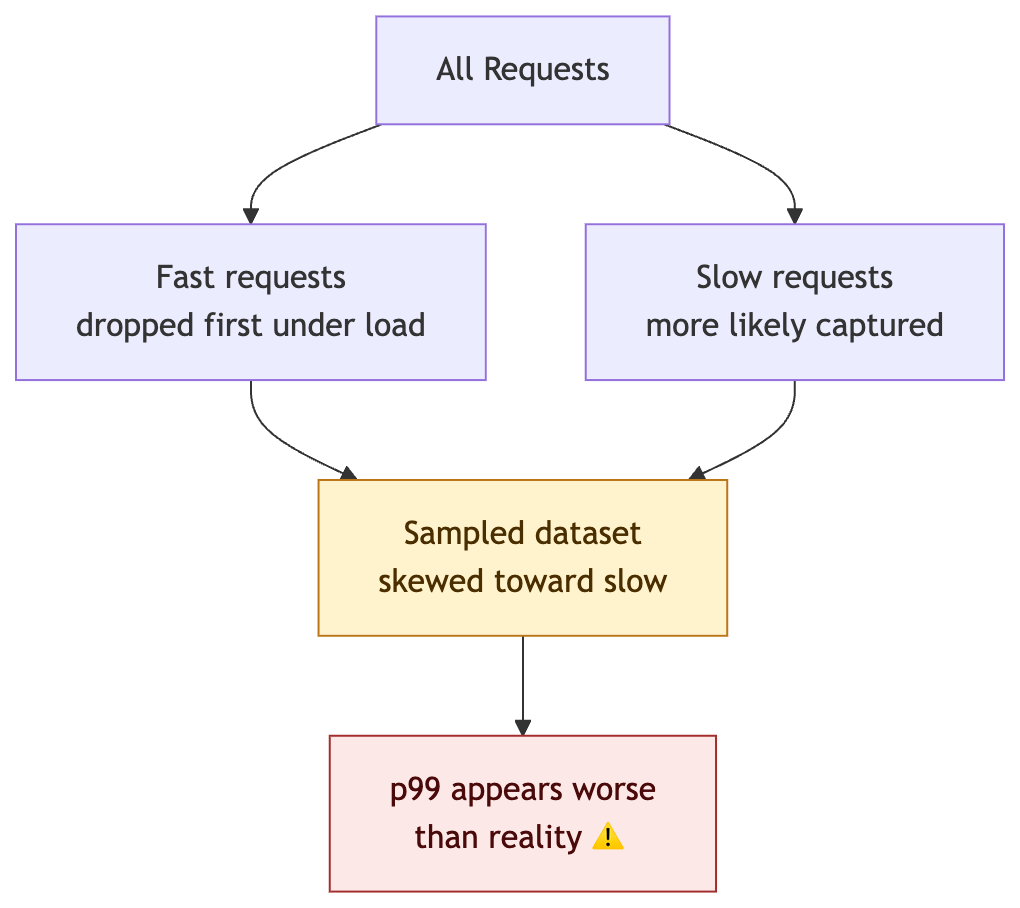
A p99 of 200ms from 100 samples tells you almost nothing. A p99 of 200ms from 1M samples is a production signal you can act on.
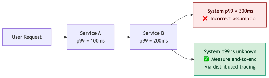
Why You Cannot Average Percentiles
This is one of the most common — and most costly — mistakes in distributed systems monitoring.
You cannot add or average percentiles across services. They do not compose linearly.
Tail latency amplifies non-linearly due to three compounding effects:
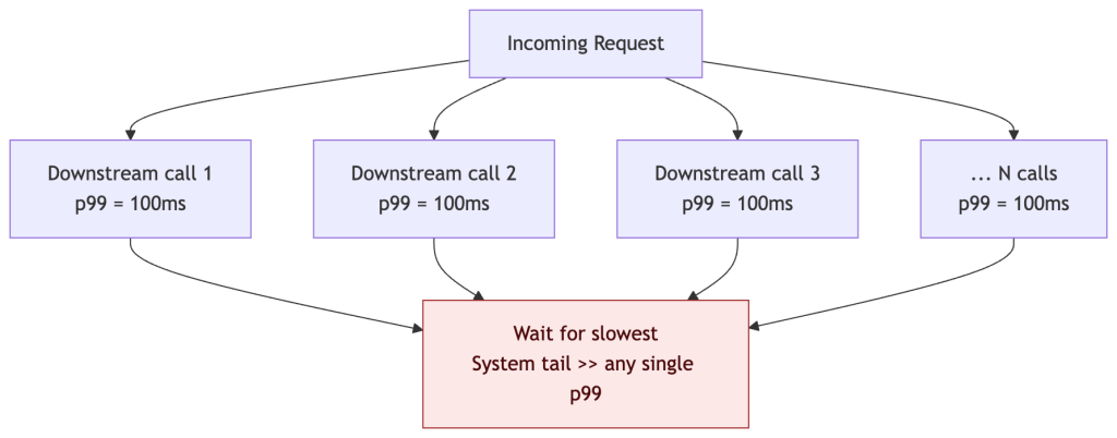
Fanout Amplification
When a request fans out to N parallel downstream calls, the response time is gated by the slowest response. The probability that at least one call exceeds the p99 threshold grows quickly with fanout width:
| Parallel Calls | P(at least one slow) | Effective impact |
|---|---|---|
| 1 call, p99=100ms | 1% chance | Tail as expected |
| 5 calls, p99=100ms | ~4.9% chance | p99 now hits ~p95 of any one call |
| 10 calls, p99=100ms | ~9.6% chance | What was p99 is now your p90 |
| 50 calls, p99=100ms | ~39% chance | Tail latency dominates the system |
Formula:
P(at least one slow) = 1 - (1 - p)^Nwherep= tail probability (0.01 for p99) andN= fanout width. At N=50, nearly 4 in 10 requests hit the tail — even if every individual service looks healthy.
Retries Under Load
Retries multiply load in the worst possible moment:
| Retry count | Effective load multiplier |
|---|---|
| 0 retries | 1x |
| 1 retry | up to 2x |
| 2 retries | up to 3x |
Under saturation this creates a positive feedback loop: slow responses trigger retries → retries increase load → load increases slowness → more retries. A naive retry strategy on a service already at 90% capacity can push it past the saturation point entirely, collapsing tail latency for all users — the opposite of the intended effect.
Mitigate with exponential backoff + jitter, retry budgets, and circuit breakers that stop retrying once a threshold of failures is reached.
Queuing Effects
Under load, requests queue before being served. Queue wait time compounds with service latency — and per-service percentiles capture neither the queue depth nor the interaction between the two.
The only reliable way to measure end-to-end tail latency in a distributed system is distributed tracing — measuring at the request boundary, not at each service in isolation.
Per-Service vs End-to-End Percentiles
This distinction is often overlooked and frequently causes monitoring blind spots.
| Measurement | Question it answers | Limitation |
|---|---|---|
| Per-service p99 | “Is this service healthy?” | Cannot see interactions between services |
| End-to-end p99 | “Is the user experience healthy?” | Requires tracing infrastructure |
A system can have perfectly healthy per-service p99s and still deliver terrible end-to-end latency — because fanout, retries, and queuing effects are invisible at the individual service level.
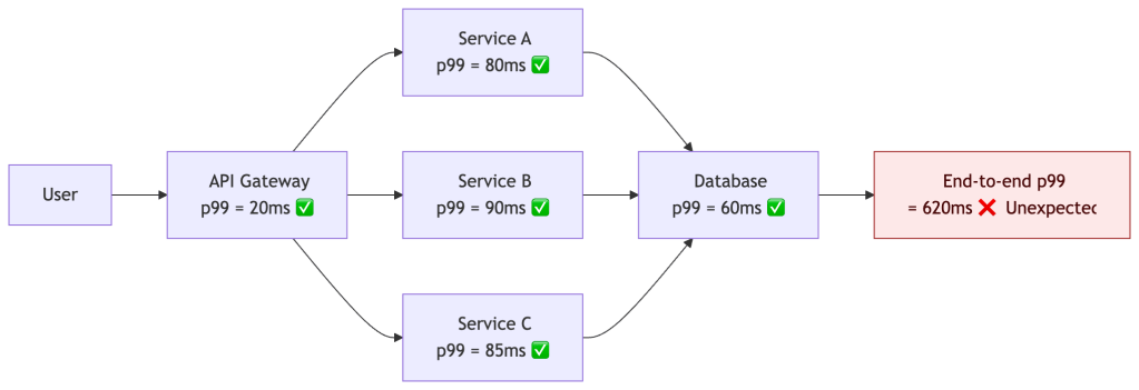
Every hop looks healthy individually. The user experience is not. This is why distributed tracing is not optional at scale — it’s the only way to see what the user actually sees.
Latency vs Throughput: The Fundamental Tradeoff
Optimizing for tail latency almost always reduces maximum throughput. This is not a bug — it’s a design choice that needs to be made explicitly.
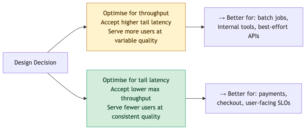
Concretely:
- Aggressive timeouts → better p99, but more failed requests at the margin
- Load shedding → protects the tail, but some requests are dropped entirely
- Hedged requests → cuts tail latency, but doubles downstream load for those requests
There is no free lunch. Committing to a p99 SLO is implicitly committing to a throughput ceiling. Make that tradeoff visible in your architecture design docs, not just your dashboards.
Designing for Tail Latency
Understanding percentiles should drive design decisions, not just dashboards. Common techniques for reducing p99:
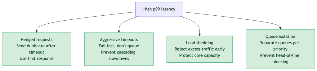
Key principle: Optimizing p50 rarely improves user experience at scale. The users most at risk of churning are in your tail — optimizing p99 is where reliability work has the highest business leverage.
Percentiles in SLO Design
SLAs are binary commitments. SLOs (Service Level Objectives) are the internal engineering targets that give you room to operate safely — and they’re always expressed in percentiles.
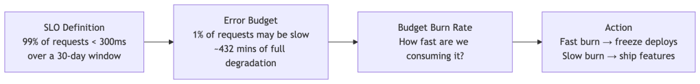
The error budget model lets you answer the question: “Can we ship this risky change?” — not with gut feel, but with a measurable runway. A fast-burning error budget means freeze; a healthy budget means velocity.
Alert on SLO burn rate, not on raw percentile thresholds. A p99 of 400ms on a Sunday at 2am with 100 requests is very different from a p99 of 400ms on a Monday at 10am with 50,000 requests.
Practical Reference
| Percentile | Who It Protects | Minimum Sample Size | Use It For |
|---|---|---|---|
| p50 | The typical user | 100+ | General UX quality, capacity planning |
| p95 | 1 in 20 tail users | 500+ | Reliability targets, SLA commitments |
| p99 | 1 in 100 tail users | 1,000+ | Catching serious outliers, SLO tracking |
| p99.9 | 1 in 1000 tail users | 10,000+ | High-traffic, payment-critical paths |
Before and After a Performance Fix
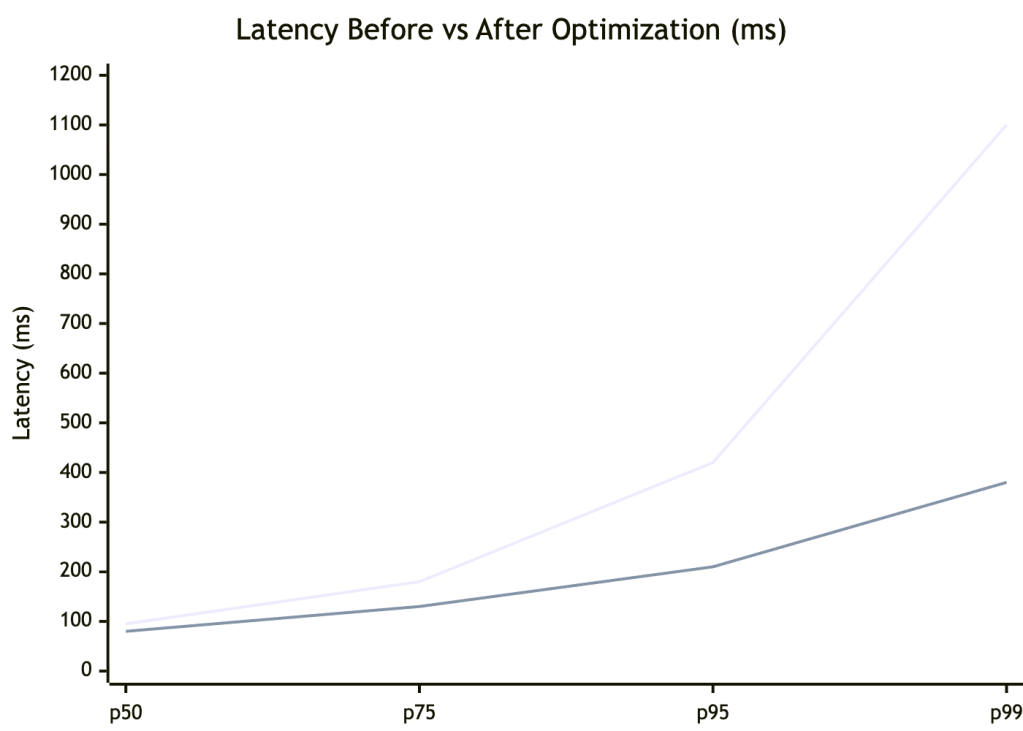
The optimization improved all percentiles — but the biggest win was at p99, dropping from 1,100ms to 380ms (~3x). p50 improved modestly (95ms → 80ms). This is the typical pattern: tail improvements have outsized impact on user experience and error budgets.
Production Checklist
Before shipping percentile-based monitoring to production, validate each of these:
- [ ] Tracking p50, p95, p99 at minimum — p99.9 for critical paths
- [ ] Sample size is sufficient for statistical stability (see table above)
- [ ] Using histograms, not averages or legacy summaries
- [ ] Aggregation is correct — not averaging percentiles across instances
- [ ] Monitoring per-endpoint, not just global service-level rollups
- [ ] Correlating spikes with traces and logs, not just metrics
- [ ] Alerting on SLO burn rate, not absolute percentile thresholds
- [ ] Load testing tool uses coordinated omission correction (e.g.
wrk2,Gatling) - [ ] Sampling strategy does not bias toward slow requests under load
- [ ] Metrics cost (cardinality, storage, CPU) is accounted for — high-resolution histograms are not free
Summary
Percentiles are not just a measurement tool — they’re a design constraint, a contractual unit, and a user empathy instrument.
- Averages lie. Percentiles surface what averages bury.
- Tail latency compounds across services in ways simple arithmetic cannot predict.
- Your computation method matters — a histogram p99 and a t-digest p99 are not the same number.
- Sample size determines signal. Low-volume p99s are noise.
- SLOs + error budgets turn percentiles into engineering decisions, not just monitoring numbers.
- Per-service p99s can all be green while end-to-end p99 is red. Trace, don’t assume.
- Tail latency and throughput trade off. Make that choice deliberately.
- Optimise the tail. That’s where users churn, SLAs break, and reputations are made.
“Your average user doesn’t exist. Your p99 user is the one writing the one-star review.”

Leave a comment