Understanding Amazon Dynamo: A Deep Dive into Distributed System Design

A senior engineer’s perspective on building highly available distributed systems

This is a long-form reference — every section stands on its own, so feel free to jump directly to whatever is most relevant to you.

Introduction: Why Dynamo Changed Everything

When Amazon published the Dynamo paper in 2007, it wasn’t just another academic exercise. It was a battle-tested solution to real problems at massive scale. I remember when I first read this paper—it fundamentally changed how I thought about distributed systems.

Dynamo is a distributed key-value storage system. It was designed to support Amazon’s high-traffic services such as the shopping cart and session management systems. There are no secondary indexes, no joins, no relational semantics—just keys and values, with extreme focus on availability and scalability. It does not provide linearizability or global ordering guarantees, even at the highest quorum settings. If your system requires those properties, Dynamo is not the right tool.

The core problem Amazon faced was simple to state but brutal to solve: How do you build a storage system that never says “no” to customers? When someone tries to add an item to their shopping cart during a network partition or server failure, rejecting that write isn’t acceptable. Every lost write is lost revenue and damaged customer trust.

The CAP Theorem Trade-off: Why Dynamo Chooses Availability

Before diving into how Dynamo works, you need to understand the fundamental constraint it’s designed around.

What is CAP Theorem?

The CAP theorem describes a fundamental trade-off in distributed systems: when a network partition occurs, you must choose between consistency and availability. The three properties are:

Consistency (C): All nodes see the same data at the same time
Availability (A): Every request gets a response (success or failure)
Partition Tolerance (P): System continues working despite network failures

A common shorthand is “pick 2 of 3,” but this is an oversimplification. In practice, network partitions are unavoidable at scale, so the real decision is: when partitions occur (and they will), do you sacrifice consistency or availability? That’s the actual design choice.

The harsh reality: Network partitions WILL happen. Cables get cut, switches fail, datacenters lose connectivity. You can’t avoid them, so you must choose: Consistency or Availability?

Traditional Databases Choose Consistency

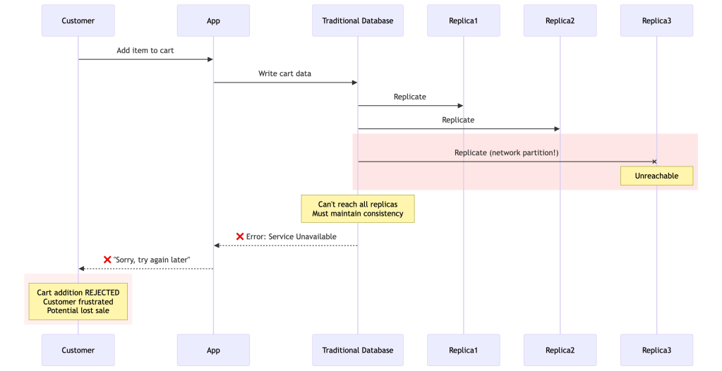
Traditional approach:

			
Database: "I can't guarantee all replicas are consistent,
           so I'll reject your write to be safe."
Result: Customer sees error, cart is empty
Impact: Lost revenue, poor experience

Dynamo Chooses Availability

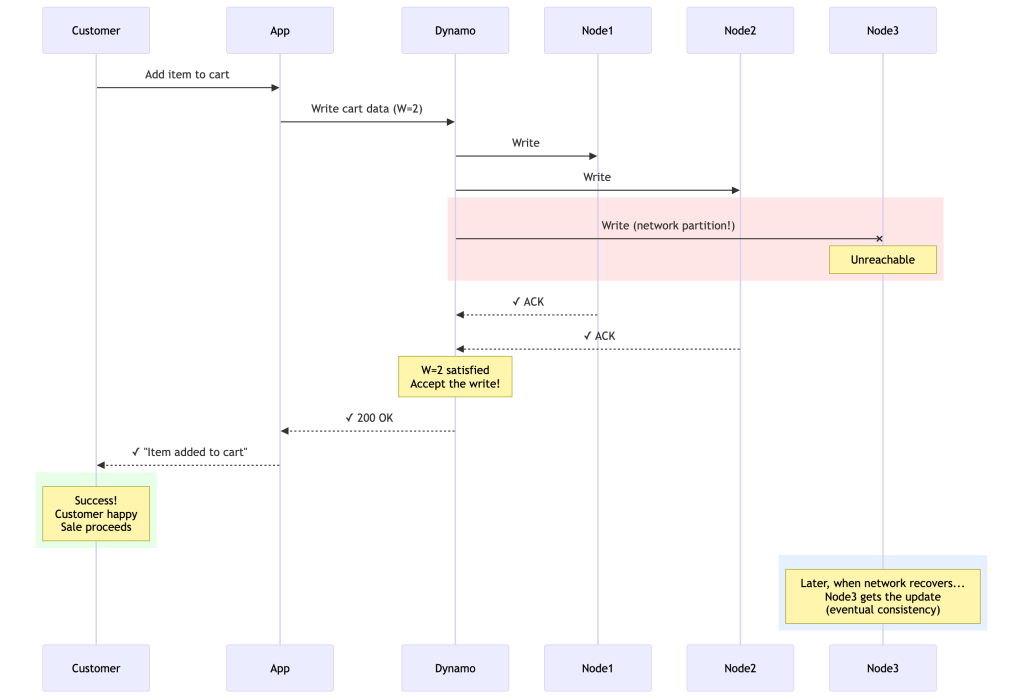
Dynamo’s approach:

			
Dynamo: "I'll accept your write with the replicas I can reach.
         The unreachable replica will catch up later."
Result: Customer sees success, item in cart
Impact: Sale continues, happy customer

The Trade-off Visualized

			
When a partition occurs:
Traditional Database: Choose C over A → Sacrifice Availability
- ✓ All replicas always have same data
- ✓ No conflicts to resolve
- ❌ Rejects writes during failures
- ❌ Poor customer experience
- ❌ Lost revenue
Dynamo:              Choose A over C → Sacrifice Strong Consistency
- ✓ Accepts writes even during failures
- ✓ Excellent customer experience
- ✓ No lost revenue
- ❌ Replicas might temporarily disagree
- ❌ Application must handle conflicts

		

Real Amazon Example: Black Friday Shopping Cart

Imagine it’s Black Friday. Millions of customers are shopping. A network cable gets cut between datacenters.

With traditional database:

			
Time: 10:00 AM - Network partition occurs
Result: 
- All shopping cart writes fail
- "Service Unavailable" errors
- Customers can't checkout
- Twitter explodes with complaints
- Estimated lost revenue: $100,000+ per minute

		

With Dynamo:

			
Time: 10:00 AM - Network partition occurs
Result:
- Shopping cart writes continue
- Customers see success
- Some carts might have conflicts (rare)
- Application merges conflicting versions
- Estimated lost revenue: $0
- A few edge cases need conflict resolution (acceptable)

		

Why This Choice Makes Sense for E-commerce

Amazon did the math:

Cost of rejecting a write: Immediate lost sale ($50-200)
Cost of accepting a conflicting write: Occasionally need to merge shopping carts (rarely happens, easily fixable)
Business decision: Accept writes, deal with rare conflicts

Types of data where Availability > Consistency:

Shopping carts (merge conflicting additions)
Session data (last-write-wins is fine)
User preferences (eventual consistency acceptable)
Best seller lists (approximate is fine)

Types of data where Consistency > Availability:

Bank account balances (can’t have conflicting balances)
Inventory counts (can’t oversell)
Transaction logs (must be ordered)

This is why Dynamo isn’t for everything—but for Amazon’s e-commerce use cases, choosing availability over strong consistency was the right trade-off.

Important nuance: While Dynamo is often described as an AP system, it’s more accurate to call it a tunable consistency system. Depending on your R and W quorum configuration, it can behave closer to CP. The AP label applies to its default/recommended configuration optimized for e-commerce workloads.

Core Architecture Components

1. Consistent Hashing for Partitioning

Let me explain this with a concrete example, because consistent hashing is one of those concepts that seems magical until you see it in action.

The Problem: Traditional Hash-Based Sharding

Imagine you have 3 servers and want to distribute data across them. The naive approach:

			
# Traditional approach - DON'T DO THIS
def get_server(key, num_servers):
    hash_value = hash(key)
    return hash_value % num_servers  # Modulo operation
# With 3 servers:
get_server("user_123", 3)  # Returns server 0
get_server("user_456", 3)  # Returns server 1
get_server("user_789", 3)  # Returns server 2

		

This works… until you add or remove a server. Let’s see what happens when we go from 3 to 4 servers:

			
# Before (3 servers):
"user_123" → hash % 3 = 0 → Server 0
"user_456" → hash % 3 = 1 → Server 1
"user_789" → hash % 3 = 2 → Server 2
# After (4 servers):
"user_123" → hash % 4 = 0 → Server 0 ✓ (stayed)
"user_456" → hash % 4 = 1 → Server 1 ✓ (stayed)
"user_789" → hash % 4 = 2 → Server 2 ✓ (stayed)
# But wait - this is lucky! In reality, most keys MOVE:
"product_ABC" → hash % 3 = 2 → Server 2
"product_ABC" → hash % 4 = 3 → Server 3 ✗ (MOVED!)

		

The disaster: When you change the number of servers, nearly ALL your data needs to be redistributed. Imagine moving terabytes of data just to add one server!

The Solution: Consistent Hashing

Consistent hashing solves this by treating the hash space as a circle (0 to 2^32 – 1, wrapping around).

Step 1: Place servers on the ring

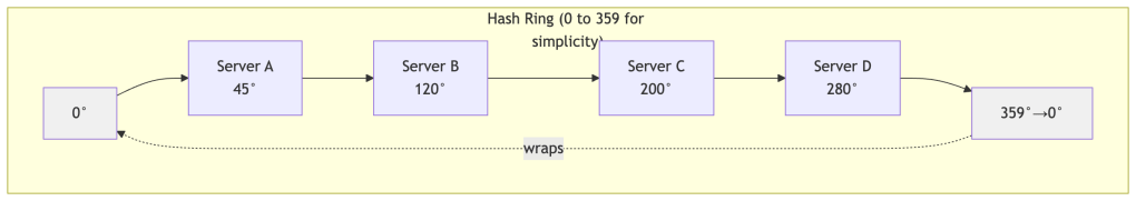
Each server is assigned a random position on the ring (called a “token”). Think of this like placing markers on a circular racetrack.

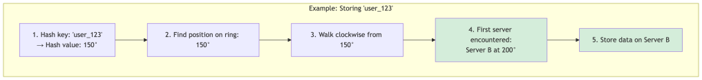
Step 2: Place data on the ring

When you want to store data, you:

Hash the key to get a position on the ring
Walk clockwise from that position
Store the data on the first server you encounter

Visual Example: Complete Ring

Here’s the ring laid out in order. Keys walk clockwise to the next server:

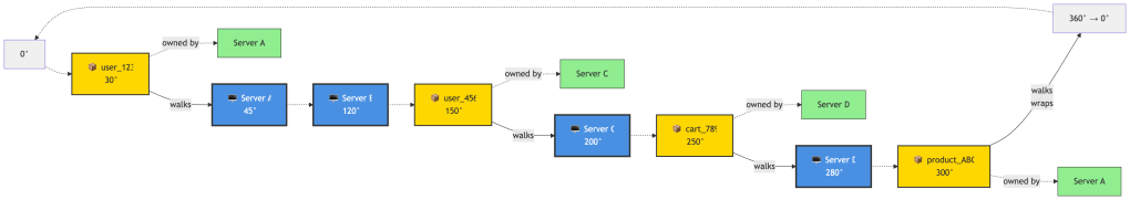
Simple rule: A key walks clockwise until it hits a server. That server owns the key.

Examples:

user_123 at 30° → walks to 45° → Server A owns it
user_456 at 150° → walks to 200° → Server C owns it
cart_789 at 250° → walks to 280° → Server D owns it
product_ABC at 300° → walks past 360°, wraps to 0°, continues to 45° → Server A owns it

Who owns what range?

Server A (45°): owns everything from 281° to 45° (wraps around)
Server B (120°): owns everything from 46° to 120°
Server C (200°): owns everything from 121° to 200°
Server D (280°): owns everything from 201° to 280°

The Magic: Adding a Server

Now let’s see why this is brilliant. We add Server E at position 160°:

			
BEFORE:
Server A (45°)  → owns 281°-45°
Server B (120°) → owns 46°-120°
Server C (200°) → owns 121°-200°  ← THIS RANGE WILL SPLIT
Server D (280°) → owns 201°-280°
AFTER:
Server A (45°)  → owns 281°-45°   ← NO CHANGE
Server B (120°) → owns 46°-120°   ← NO CHANGE
Server E (160°) → owns 121°-160°  ← NEW! Takes part of C's range
Server C (200°) → owns 161°-200°  ← SMALLER range
Server D (280°) → owns 201°-280°  ← NO CHANGE

		

Result: Only keys in range 121°-160° need to move (from C to E). Servers A, B, and D are completely unaffected!

The Virtual Nodes Optimization

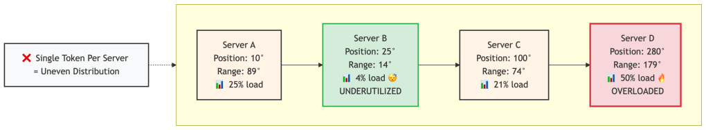
There’s a critical problem with the basic consistent hashing approach: random distribution can be extremely uneven.

The Problem in Detail:

When you randomly assign one position per server, you’re essentially throwing darts at a circular board. Sometimes the darts cluster together, sometimes they spread out. This creates hotspots.

Let me show you a concrete example:

			
Scenario: 4 servers with single random tokens
Server A: 10°   }
Server B: 25°   } ← Only 75° apart! Tiny ranges
Server C: 100°  }
Server D: 280°  ← 180° away from C! Huge range
Range sizes:
- Server A owns: 281° to 10° = 89° (25% of ring)
- Server B owns: 11° to 25° = 14° (4% of ring)  ← Underutilized!
- Server C owns: 26° to 100° = 74° (21% of ring)
- Server D owns: 101° to 280° = 179° (50% of ring)  ← Overloaded!

		

Real-world consequences:

Uneven load: Server D handles 50% of all data while Server B handles only 4%. This means:

Server D’s CPU, disk, and network are maxed out
Server B is mostly idle (wasted capacity)
Your 99.9th percentile latency is dominated by Server D being overloaded

Hotspot cascading: When Server D becomes slow or fails:

All its 50% load shifts to Server A (the next one clockwise)
Server A now becomes overloaded
System performance degrades catastrophically

Inefficient scaling: Adding servers doesn’t help evenly because new servers might land in already small ranges

Visualizing the problem:

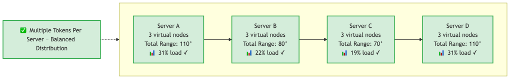
Dynamo’s solution: Each physical server gets multiple virtual positions (tokens).

Instead of one dart throw per server, throw many darts. The more throws, the more even the distribution becomes (law of large numbers).

How Virtual Nodes Fix the Problem:

Let’s take the same 4 servers, but now each server gets 3 virtual nodes (tokens) instead of 1:

			
Physical Server A gets 3 tokens: 10°, 95°, 270°
Physical Server B gets 3 tokens: 25°, 180°, 310°
Physical Server C gets 3 tokens: 55°, 150°, 320°
Physical Server D gets 3 tokens: 75°, 200°, 340°
Now the ring looks like:
10° A, 25° B, 55° C, 75° D, 95° A, 150° C, 180° B, 200° D, 270° A, 310° B, 320° C, 340° D
Range sizes (approximately):
- Server A total: 15° + 55° + 40° = 110° (31% of ring)
- Server B total: 30° + 20° + 30° = 80° (22% of ring)
- Server C total: 20° + 30° + 20° = 70° (19% of ring)
- Server D total: 20° + 70° + 20° = 110° (31% of ring)

		

Much better! Load ranges from 19% to 31% instead of 4% to 50%.

Why this works:

Statistics: With more samples (tokens), the random distribution averages out. This is the law of large numbers in action.
Granular load distribution: When a server fails, its load is distributed across many servers, not just one neighbor:

   Server A fails:
   - Its token at 10° → load shifts to Server B's token at 25°
   - Its token at 95° → load shifts to Server C's token at 150°
   - Its token at 270° → load shifts to Server B's token at 310°

   Result: The load is spread across multiple servers!

Smooth scaling: When adding a new server with 3 tokens, it steals small amounts from many servers instead of a huge chunk from one server.

Real Dynamo configurations:

The paper mentions different strategies evolved over time. In production:

Early versions: 100-200 virtual nodes per physical server
Later optimized to: Q/S tokens per node (where Q = total partitions, S = number of servers)
Typical setup: Each physical server might have 128-256 virtual nodes

The Trade-off: Balance vs Overhead

More virtual nodes means better load distribution, but there’s a cost.

What you gain with more virtual nodes:

			
With 1 token per server (4 servers):
Load variance: 4% to 50% (±46% difference) ❌
With 3 tokens per server (12 virtual nodes):
Load variance: 19% to 31% (±12% difference) ✓
With 128 tokens per server (512 virtual nodes):
Load variance: 24% to 26% (±2% difference) ✓✓

		

What it costs:

Metadata size: Each node maintains routing information

1 token per server: Track 4 entries
128 tokens per server: Track 512 entries

Gossip overhead: Nodes exchange membership info periodically

More tokens = more data to sync between nodes
Every second, nodes gossip their view of the ring

Rebalancing complexity: When nodes join/leave

More virtual nodes = more partition transfers to coordinate
But each transfer is smaller (which is actually good for bootstrapping)

Dynamo’s evolution:

The paper describes how Amazon optimized this over time:

			
Strategy 1 (Initial):
- 100-200 random tokens per server
- Problem: Huge metadata (multiple MB per node)
- Problem: Slow bootstrapping (had to scan for specific key ranges)
Strategy 3 (Current):
- Q/S tokens per server (Q=total partitions, S=number of servers)
- Equal-sized partitions
- Example: 1024 partitions / 8 servers = 128 tokens per server
- Benefit: Metadata reduced to KB
- Benefit: Fast bootstrapping (transfer whole partition files)

		

Real production sweet spot:

Most Dynamo deployments use 128-256 virtual nodes per physical server. This achieves:

Load distribution within 10-15% variance (good enough)
Metadata overhead under 100KB per node (negligible)
Fast failure recovery (load spreads across many nodes)

Why not more? Diminishing returns. Going from 128 to 512 tokens only improves load balance by 2-3%, but doubles metadata size and gossip traffic.

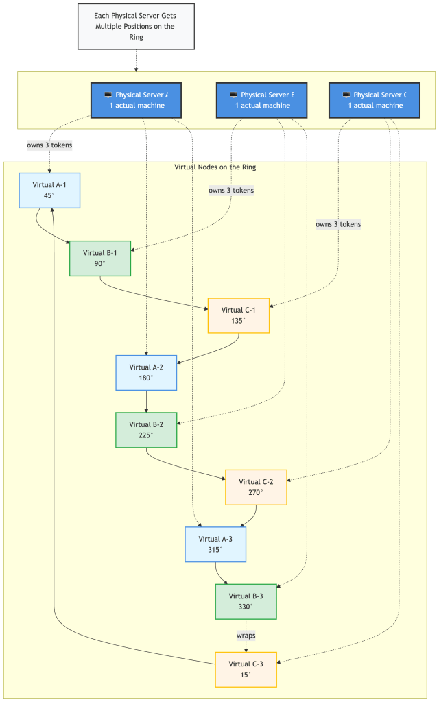
Key concept: Physical servers (top) map to multiple virtual positions (bottom) on the ring. This distributes each server’s load across different parts of the hash space.

Benefits:

More even load distribution
When a server fails, its load is distributed across many servers (not just one neighbor)
When a server joins, it steals a small amount from many servers

Real-World Impact Comparison

Let’s see the difference with real numbers:

			
Traditional Hashing (3 servers → 4 servers):
- Keys that need to move: ~75% (3 out of 4)
- Example: 1 million keys → 750,000 keys must migrate
Consistent Hashing (3 servers → 4 servers):
- Keys that need to move: ~25% (1 out of 4)
- Example: 1 million keys → 250,000 keys must migrate
With Virtual Nodes (150 vnodes total → 200 vnodes):
- Keys that need to move: ~12.5% (spread evenly)
- Example: 1 million keys → 125,000 keys must migrate
- Load is balanced across all servers

		

The “Aha!” Moment

The key insight is this: Consistent hashing decouples the hash space from the number of servers.

Traditional: server = hash(key) % num_servers ← num_servers is in the formula!
Consistent: server = ring.findNextClockwise(hash(key)) ← num_servers isn’t in the formula!

This is why adding/removing servers only affects a small portion of the data. The hash values don’t change—only which server “owns” which range changes, and only locally.

Think of it like a circular running track with water stations (servers). If you add a new water station, runners only change stations if they’re between the old nearest station and the new one. Everyone else keeps going to their same station.

2. Replication Strategy (N, R, W)

The Problem: Availability vs Consistency Trade-off

Imagine you’re building Amazon’s shopping cart. A customer adds an item to their cart, but at that exact moment:

One server is being rebooted for maintenance
Another server has a network hiccup
A third server is perfectly fine

Traditional database approach (strong consistency):

			
Client: "Add this item to my cart"
Database: "I need ALL replicas to confirm before I say yes"
Server 1: ✗ (rebooting)
Server 2: ✗ (network issue)
Server 3: ✓ (healthy)
Result: "Sorry, service unavailable. Try again later."

		

Customer experience: 😡 “I can’t add items to my cart during Black Friday?!”

This is unacceptable for e-commerce. Every rejected write is lost revenue.

Dynamo’s Solution: Tunable Quorums

Dynamo gives you three knobs to tune the exact trade-off you want:

N: Number of replicas (how many copies of the data)
R: Read quorum (how many replicas must respond for a successful read)
W: Write quorum (how many replicas must acknowledge for a successful write)

The magic formula: When R + W > N, you guarantee quorum overlap—meaning at least one node that received the write will be queried during any read. This overlap enables detection of the latest version, provided the reconciliation logic correctly identifies the highest vector clock. It does not automatically guarantee read-your-writes unless the coordinator properly resolves versions.

Let me show you why this matters with real scenarios:

Scenario 1: Shopping Cart (Prioritize Availability)

			
N = 3  # Three replicas for durability
R = 1  # Read from any single healthy node
W = 1  # Write to any single healthy node
# Trade-off analysis:
# ✓ Writes succeed even if 2 out of 3 nodes are down
# ✓ Reads succeed even if 2 out of 3 nodes are down
# ✓ Maximum availability - never reject customer actions
# ✗ Might read stale data
# ✗ Higher chance of conflicts (but we can merge shopping carts)

		

What happens during failure:

			
Client: "Add item to cart"
Coordinator tries N=3 nodes:
- Node 1: ✗ Down
- Node 2: ✓ ACK (W=1 satisfied!)
- Node 3: Still waiting...
Result: SUCCESS returned to client immediately
Node 3 eventually gets the update (eventual consistency)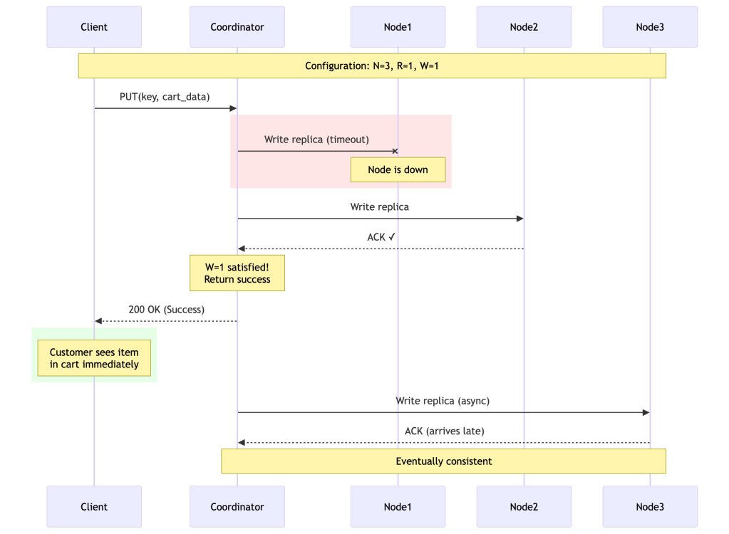

		

Scenario 2: Session State (Balanced Approach)

			
N = 3
R = 2  # Must read from 2 nodes
W = 2  # Must write to 2 nodes
# Trade-off analysis:
# ✓ R + W = 4 > N = 3 → Read-your-writes guaranteed
# ✓ Tolerates 1 node failure
# ✓ Good balance of consistency and availability
# ✗ Write fails if 2 nodes are down
# ✗ Read fails if 2 nodes are down

		

Why R + W > N enables read-your-writes:

			
Write to W=2 nodes: [A, B]
Later, read from R=2 nodes: [B, C]
Because W + R = 4 > N = 3, there's guaranteed overlap!
At least one node (B in this case) will have the latest data.
The coordinator detects the newest version by comparing vector clocks.
This guarantees seeing the latest write as long as reconciliation
picks the causally most-recent version correctly.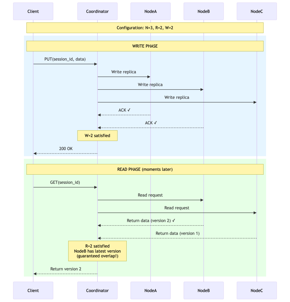

		

Scenario 3: Financial Data (Prioritize Consistency)

			
N = 3
R = 3  # Must read from ALL nodes
W = 3  # Must write to ALL nodes
# Trade-off analysis:
# ✓ Full replica quorum — reduces likelihood of divergent versions
# ✓ Any read will overlap every write quorum
# ✗ Write fails if ANY node is down
# ✗ Read fails if ANY node is down
# ✗ Poor availability during failures

		

Systems requiring strict transactional guarantees typically choose CP systems instead. This configuration is technically supported by Dynamo but sacrifices the availability properties that motivate using it in the first place.

Configuration Comparison Table

Config	N	R	W	Availability	Consistency	Use Case
High Availability	3	1	1	⭐⭐⭐⭐⭐	⭐⭐	Shopping cart, wish list
Balanced	3	2	2	⭐⭐⭐⭐	⭐⭐⭐⭐	Session state, user preferences
Full Quorum	3	3	3	⭐⭐	⭐⭐⭐⭐⭐	High-stakes reads (not linearizable)
Read-Heavy	3	1	3	⭐⭐⭐ (reads)	⭐⭐⭐⭐	Product catalog, CDN metadata
Write-Heavy	3	3	1	⭐⭐⭐ (writes)	⭐⭐⭐	Click tracking, metrics

Note on financial systems: Systems requiring strong transactional guarantees (e.g., bank account balances) typically shouldn’t use Dynamo. That said, some financial systems do build on Dynamo-style storage for their persistence layer while enforcing stronger semantics at the application or business logic layer.

The Key Insight

Most systems use N=3, R=2, W=2 because:

Durability: Can tolerate up to 2 replica failures before permanent data loss (assuming independent failures and no correlated outages).
Availability: Tolerates 1 node failure for both reads and writes
Consistency: R + W > N guarantees that read and write quorums overlap, enabling read-your-writes behavior in the absence of concurrent writes.
Performance: Don’t wait for the slowest node (only need 2 out of 3)

Real production numbers from the paper:

Amazon’s shopping cart service during peak (holiday season):

Configuration: N=3, R=2, W=2
Handled tens of millions of requests
Over 3 million checkouts in a single day
No downtime, even with server failures

This tunable approach is what made Dynamo revolutionary. You’re not stuck with one-size-fits-all—you tune it based on your actual business requirements.

3. Vector Clocks for Versioning

The Problem: Detecting Causality in Distributed Systems

When multiple nodes can accept writes independently, you need to answer a critical question: Are these two versions of the same data related, or were they created concurrently?

Why timestamps don’t work:

			
Scenario: Two users edit the same shopping cart simultaneously
User 1 at 10:00:01.500 AM: Adds item A → Writes to Node X
User 2 at 10:00:01.501 AM: Adds item B → Writes to Node Y
Physical timestamp says: User 2's version is "newer"
Reality: These are concurrent! Both should be kept!
Problem: 
- Clocks on different servers are NEVER perfectly synchronized
- Clock skew can be seconds or even minutes
- Network delays are unpredictable
- Physical time doesn't capture causality

		

What we really need to know:

			
Version A happened before Version B?     → B can overwrite A
Version A and B are concurrent?          → Keep both, merge later
Version A came from reading Version B?   → We can track this!

The Solution: Vector Clocks

A vector clock is a simple data structure: a list of (node_id, counter) pairs that tracks which nodes have seen which versions.

The rules:

When a node writes data, it increments its own counter
When a node reads data, it gets the vector clock
When comparing two vector clocks:

If all counters in A ≤ counters in B → A is an ancestor of B (B is newer)
If some counters in A > B and some B > A → A and B are concurrent (conflict!)

Step-by-Step Example

Let’s trace a shopping cart through multiple updates:

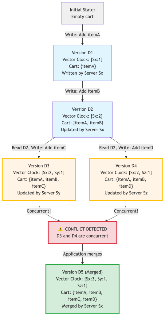
Breaking down the conflict:

			
D3: [Sx:2, Sy:1]  vs  D4: [Sx:2, Sz:1]
Comparing:
- Sx: 2 == 2  ✓ (equal)
- Sy: 1 vs missing in D4  → D3 has something D4 doesn't
- Sz: missing in D3 vs 1  → D4 has something D3 doesn't
Conclusion: CONCURRENT! Neither is an ancestor of the other.
Both versions must be kept and merged.

		

Real-World Characteristics

The Dynamo paper reports the following conflict distribution measured over 24 hours of Amazon’s production shopping cart traffic. These numbers reflect Amazon’s specific workload — high read/write ratio, mostly single-user sessions — and should not be assumed to generalize to all Dynamo deployments:

			
94%    - Single version (no conflict)
00057%  - 2 versions
00047%  - 3 versions  
00009%  - 4 versions

Key insight: Conflicts are RARE in practice!

Why conflicts happen:

Not usually from network failures
Mostly from concurrent writers (often automated processes/bots)
Human users rarely create conflicts because they’re slow compared to network speed

The Size Problem

Vector clocks can grow unbounded if many nodes coordinate writes. Dynamo’s solution: truncate the oldest entries once the clock exceeds a size threshold.

			
// When vector clock exceeds threshold (e.g., 10 entries)
// Remove the oldest entry based on wall-clock timestamp
vectorClock = {
  'Sx': {counter: 5, timestamp: 1609459200},
  'Sy': {counter: 3, timestamp: 1609459800},
  'Sz': {counter: 2, timestamp: 1609460400},
  // ... 10 more entries
}
// If size > 10, remove entry with oldest timestamp
// ⚠ Risk: Dropping an entry collapses causality information.
//   Two versions that were causally related may now appear
//   concurrent, forcing the application to resolve a conflict
//   that didn't actually exist. In practice, Amazon reports
//   this has not been a significant problem — but it is a
//   real theoretical risk in high-churn write environments
//   with many distinct coordinators.

		

4. Sloppy Quorum and Hinted Handoff

The Problem: Strict Quorums Kill Availability

Traditional quorum systems are rigid and unforgiving.

Traditional strict quorum:

			
Your data is stored on nodes: A, B, C (preference list)
Write requirement: W = 2
Scenario: Node B is down for maintenance
Coordinator: "I need to write to 2 nodes from {A, B, C}"
Tries: A ✓, B ✗ (down), C ✓
Result: SUCCESS (got 2 out of 3)
Scenario: Nodes B AND C are down
Coordinator: "I need to write to 2 nodes from {A, B, C}"
Tries: A ✓, B ✗ (down), C ✗ (down)
Result: FAILURE (only got 1 out of 3)
Customer: "Why can't I add items to my cart?!" 😡

		

The problem: Strict quorums require specific nodes. If those specific nodes are down, the system becomes unavailable.

Real scenario at Amazon:

			
Black Friday, 2:00 PM
- Datacenter 1: 20% of nodes being rebooted (rolling deployment)
- Datacenter 2: Network hiccup (1-2% packet loss)
- Traffic: 10x normal load
With strict quorum:
- 15% of write requests fail
- Customer support phones explode
- Revenue impact: Millions per hour

		

The Solution: Sloppy Quorum

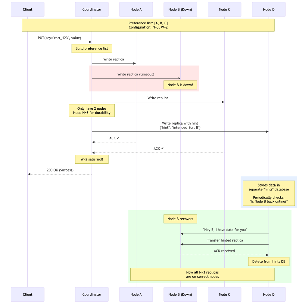
Dynamo relaxes the quorum requirement: “Write to the first N healthy nodes in the preference list, walking further down the ring if needed.”

			
Preference list for key K: A, B, C
But B is down...
Sloppy Quorum says:
"Don't give up! Walk further down the ring:
 A, B, C, D, E, F, ..."
Coordinator walks until N=3 healthy nodes are found: A, C, D
(D is a temporary substitute for B)

		

How Hinted Handoff Works

When a node temporarily substitutes for a failed node, it stores a “hint” with the data.

Detailed Hinted Handoff Process

Step 1: Detect failure and substitute

			
def write_with_hinted_handoff(key, value, N, W):
    preference_list = get_preference_list(key)  # [A, B, C]
    healthy_nodes = []
    for node in preference_list:
        if is_healthy(node):
            healthy_nodes.append((node, is_hint=False))
    # If we don't have N healthy nodes, expand the list
    if len(healthy_nodes) < N:
        extended_list = get_extended_preference_list(key)
        for node in extended_list:
            if node not in preference_list and is_healthy(node):
                healthy_nodes.append((node, is_hint=True))
            if len(healthy_nodes) >= N:
                break
    # Write to first N healthy nodes
    acks = 0
    for node, is_hint in healthy_nodes[:N]:
        if is_hint:
            # Store with hint metadata
            intended_node = find_intended_node(preference_list, node)
            success = node.write_hinted(key, value, hint=intended_node)
        else:
            success = node.write(key, value)
        if success:
            acks += 1
            if acks >= W:
                return SUCCESS
    return FAILURE

		

Step 2: Background hint transfer

			
# Runs periodically on each node (e.g., every 10 seconds)
def transfer_hints():
    hints_db = get_hinted_replicas()
    for hint in hints_db:
        intended_node = hint.intended_for
        if is_healthy(intended_node):
            try:
                intended_node.write(hint.key, hint.value)
                hints_db.delete(hint)
                log(f"Successfully transferred hint to {intended_node}")
            except:
                log(f"Will retry later for {intended_node}")

		

Why This Is Brilliant

Durability maintained:

			
Even though B is down:
- We still have N=3 copies: A, C, D
- Data won't be lost even if another node fails
- System maintains durability guarantee

Availability maximized:

			
Client perspective:
- Write succeeds immediately
- No error message
- No retry needed
- Customer happy
Traditional quorum would have failed:
- Only 2 nodes available (A, C)
- Need 3 for N=3
- Write rejected
- Customer sees error

		

Eventual consistency:

			
Timeline:
T=0:    Write succeeds (A, C, D with hint)
T=0-5min: B is down, but system works fine
T=5min: B recovers
T=5min+10sec: D detects B is back, transfers hint
T=5min+11sec: B has the data, D deletes hint
Result: Eventually, all correct replicas have the data

		

Configuration Example

			
// High availability configuration
const config = {
  N: 3,           // Want 3 replicas
  W: 2,           // Only need 2 ACKs to succeed
  R: 2,           // Read from 2 nodes
  // Sloppy quorum allows expanding preference list
  sloppy_quorum: true,
  // How far to expand when looking for healthy nodes
  max_extended_preference_list: 10,
  // How often to check for hint transfers
  hint_transfer_interval: 10_seconds,
  // How long to keep trying to transfer hints
  hint_retention: 7_days
};

		

Real-World Impact

From Amazon’s production experience:

During normal operation:

Hinted handoff rarely triggered
Most writes go to preferred nodes
Hints database is mostly empty

During failures:

			
Scenario: 5% of nodes failing at any time (normal at Amazon's scale)
Without hinted handoff:
- Write success rate: 85%
- Customer impact: 15% of cart additions fail
With hinted handoff:
- Write success rate: 99.9%+
- Customer impact: Nearly zero

		

During datacenter failure:

			
Scenario: Entire datacenter unreachable (33% of nodes)
Without hinted handoff:
- Many keys would lose entire preference list
- Massive write failures
- System effectively down
With hinted handoff:
- Writes redirect to other datacenters
- Hints accumulate temporarily
- When datacenter recovers, hints transfer
- Zero customer-visible failures

		

The Trade-off

Benefits:

✓ Maximum write availability
✓ Durability maintained during failures
✓ Automatic recovery when nodes come back
✓ No manual intervention required

Costs:

✗ Temporary inconsistency (data not on “correct” nodes)
✗ Extra storage for hints database
✗ Background bandwidth for hint transfers
✗ Slightly more complex code
✗ Hinted handoff provides temporary durability, not permanent replication. If a substitute node (like D) fails before it can transfer its hint back to B, the number of true replicas drops below N until the situation resolves. This is an important edge case to understand in failure planning.

Amazon’s verdict: The availability benefits far outweigh the costs for e-commerce workloads.

Conflict Resolution: The Shopping Cart Problem

Let’s talk about the most famous example from the paper: the shopping cart. This is where rubber meets road.

What Is a Conflict (and Why Does It Happen)?

A conflict occurs when two writes happen to the same key on different nodes, without either write “knowing about” the other. This is only possible because Dynamo accepts writes even when nodes can’t communicate—which is the whole point!

Here’s a concrete sequence of events that creates a conflict:

			
Timeline:
T=0:  Customer logs in. Cart has {shoes} on all 3 nodes.
T=1:  Network partition: Node1 can't talk to Node2.
T=2:  Customer adds {jacket} on their laptop → goes to Node1.
      Cart on Node1: {shoes, jacket}   ← Vector clock: [N1:2]
T=3:  Customer adds {hat} on their phone → goes to Node2.
      Cart on Node2: {shoes, hat}      ← Vector clock: [N2:2]
T=4:  Network heals. Node1 and Node2 compare notes.
      Node1 says: "I have version [N1:2]"
      Node2 says: "I have version [N2:2]"
      Neither clock dominates the other → CONFLICT!

		

Neither version is “wrong”—both represent real actions the customer took. Dynamo’s job is to detect this situation (via vector clocks) and surface both versions to the application so the application can decide what to do.

What Does the Application Do With a Conflict?

This is the crucial part that the paper delegates to you: the application must resolve conflicts using business logic. Dynamo gives you all the concurrent versions; your code decides how to merge them.

For the shopping cart, Amazon chose a union merge: keep all items from all concurrent versions. The rationale is simple—losing an item from a customer’s cart (missing a sale) is worse than occasionally showing a stale item they already deleted.

			
Conflict versions:
  Version A (from Node1): {shoes, jacket}
  Version B (from Node2): {shoes, hat}
Merge strategy: union
  Merged cart: {shoes, jacket, hat}  ← All items preserved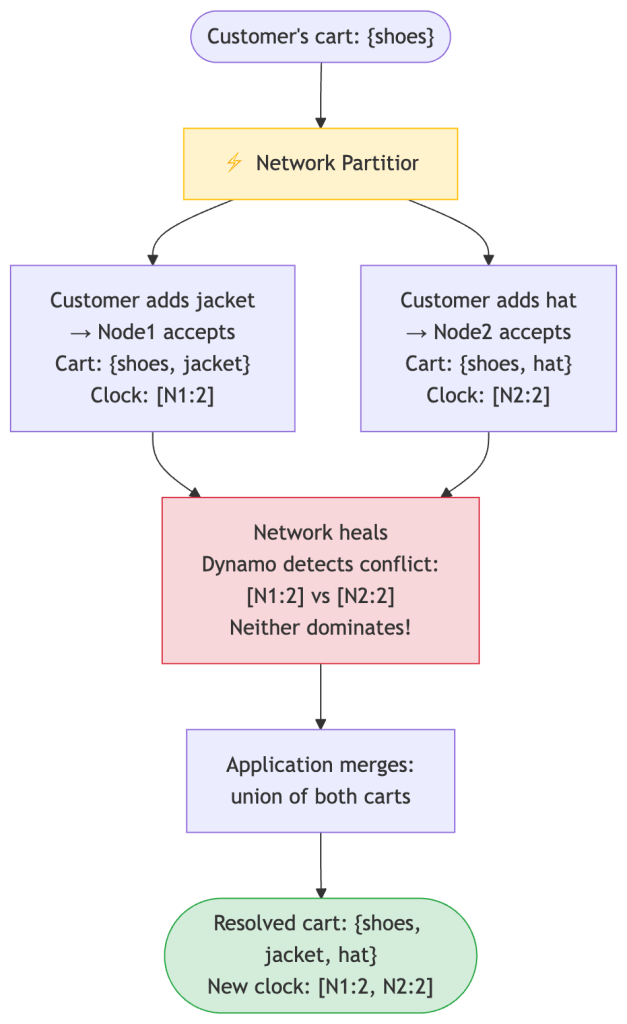

		

Here’s the actual reconciliation code:

			
from __future__ import annotations
from dataclasses import dataclass, field
class VectorClock:
    def __init__(self, clock: dict[str, int] | None = None):
        self.clock: dict[str, int] = clock.copy() if clock else {}
    def merge(self, other: "VectorClock") -> "VectorClock":
        """Merged clock = max of each node's counter across both versions."""
        all_keys = set(self.clock) | set(other.clock)
        merged = {k: max(self.clock.get(k, 0), other.clock.get(k, 0)) for k in all_keys}
        return VectorClock(merged)
    def __repr__(self):
        return f"VectorClock({self.clock})"
@dataclass
class ShoppingCart:
    items: list[str] = field(default_factory=list)
    vector_clock: VectorClock = field(default_factory=VectorClock)
    @staticmethod
    def reconcile(carts: list["ShoppingCart"]) -> "ShoppingCart":
        if len(carts) == 1:
            return carts[0]  # No conflict, nothing to do
        # Merge strategy: union of all items (never lose additions).
        # This is Amazon's choice for shopping carts.
        # A different application might choose last-write-wins or something else.
        all_items: set[str] = set()
        merged_clock = VectorClock()
        for cart in carts:
            all_items.update(cart.items)          # Union: keep everything
            merged_clock = merged_clock.merge(cart.vector_clock)
        return ShoppingCart(items=sorted(all_items), vector_clock=merged_clock)
# Example conflict scenario
cart1 = ShoppingCart(items=["shoes", "jacket"], vector_clock=VectorClock({"N1": 2}))
cart2 = ShoppingCart(items=["shoes", "hat"],    vector_clock=VectorClock({"N2": 2}))
# Dynamo detected a conflict and passes both versions to our reconcile()
reconciled = ShoppingCart.reconcile([cart1, cart2])
print(reconciled.items)  # ['hat', 'jacket', 'shoes'] — union!

		

The Deletion Problem (Why This Gets Tricky)

The union strategy has a nasty edge case: deleted items can come back from the dead.

			
T=0:  Cart: {shoes, hat}
T=1:  Customer removes hat → Cart: {shoes}           Clock: [N1:3]
T=2:  Network partition — Node2 still has old state
T=3:  Some concurrent write to Node2                  Clock: [N2:3]
T=4:  Network heals → conflict detected
T=5:  Union merge: {shoes} ∪ {shoes, hat} = {shoes, hat}
Result: Hat is BACK! Customer removed it, but it reappeared.

		

Amazon explicitly accepts this trade-off. A “ghost” item in a cart is a minor annoyance. Losing a cart addition during a Black Friday sale is lost revenue.

Engineering depth note: Merge logic must be domain-specific and carefully designed. Adding items is commutative (order doesn’t matter) and easy to merge. Removing items is not—a deletion in one concurrent branch may be silently ignored during a union-based merge. This is an intentional trade-off in Dynamo’s design, but it means the application must reason carefully about add vs. remove semantics. If your data doesn’t naturally support union merges (e.g., a counter, a user’s address), you need a different strategy—such as CRDTs, last-write-wins with timestamps, or simply rejecting concurrent writes for that data type.

Read and Write Flow

The diagrams above show the high-level flow, but let’s walk through what actually happens step-by-step during a read and a write. Understanding this concretely will make the earlier concepts click.

Write Path

Step-by-step narration of a PUT request:

Client sends the request to any node (via a load balancer) or directly to the coordinator.
The coordinator is determined — this is the first node in the preference list for the key’s hash position on the ring.
Vector clock is updated — the coordinator increments its own counter in the vector clock, creating a new version.
The coordinator writes locally, then fans out the write to the other N-1 nodes in the preference list simultaneously.
The coordinator waits for W acknowledgments. It does NOT wait for all N — just the first W to respond. The remaining nodes that haven’t responded yet will get the write eventually (or via hinted handoff if they’re down).
Once W ACKs arrive, the coordinator returns 200 OK to the client. From the client’s perspective, the write is done.

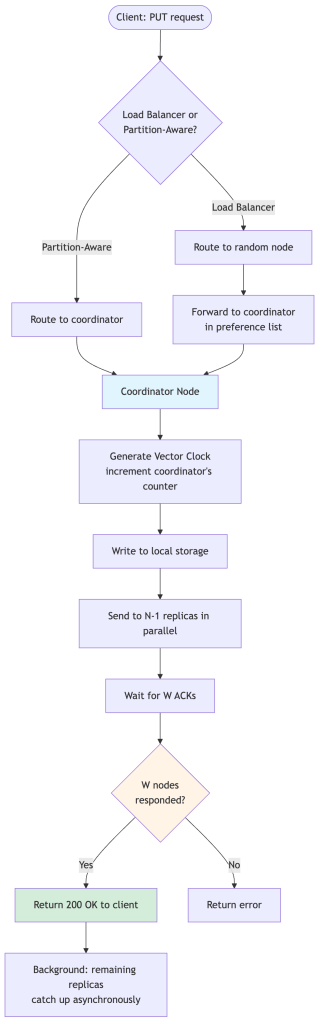
Key insight about the write path: The client gets a success response as soon as W nodes confirm. The other (N – W) nodes will receive the write asynchronously. This is why the system is “eventually consistent”—all nodes will have the data, just not necessarily at the same moment.

Read Path

Step-by-step narration of a GET request:

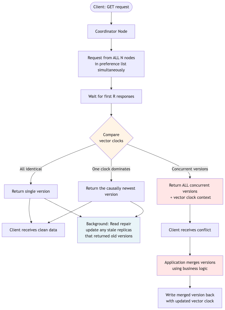
Client sends the request to the coordinator for that key.
The coordinator sends read requests to all N nodes in the preference list simultaneously (not just R). This is important — it contacts all N, but only needs R to respond.
Wait for R responses. The coordinator returns as soon as R nodes have replied, without waiting for the slower ones.
Compare the versions returned. The coordinator checks all the vector clocks:
- If all versions are identical → return the single version immediately.
- If one version’s clock dominates the others (it’s causally “newer”) → return that version.
- If versions are concurrent (neither clock dominates) → return all versions to the client, which must merge them.
Read repair happens in the background: if the coordinator noticed any node returned a stale version, it sends the latest version to that node to bring it up to date.

Why does the client receive the conflict instead of the coordinator resolving it? Because Dynamo is a general-purpose storage engine. It doesn’t know whether you’re storing a shopping cart, a user profile, or a session token. Only your application knows how to merge two conflicting versions in a way that makes business sense. The coordinator hands you the raw concurrent versions along with the vector clock context, and you do the right thing for your use case.

The vector clock context is the key to closing the loop: when the client writes the merged version back, it must include the context (the merged vector clock). This tells Dynamo that the new write has “seen” all the concurrent versions, so the conflict is resolved. Without this context, Dynamo might think it’s another concurrent write on top of the still-unresolved conflict.

Merkle Trees for Anti-Entropy

The Problem: How Do You Know When Replicas Are Out of Sync?

After a node recovers from a failure, it may have missed some writes. After a network partition heals, two replicas might diverge. How does Dynamo detect and fix these differences?

The brute-force approach would be: “Every hour, compare every key on Node A against Node B, and sync anything that’s different.” But at Amazon’s scale, a single node might store hundreds of millions of keys. Comparing them all one by one would be so slow and bandwidth-intensive that it would interfere with normal traffic.

Dynamo uses Merkle trees to solve this efficiently. The core idea: instead of comparing individual keys, compare hashes of groups of keys. If the hash matches, that whole group is identical—skip it. Only drill down into groups where hashes differ.

Important: Merkle tree sync is a background anti-entropy mechanism. It’s not on the hot read/write path. Normal reads and writes use vector clocks and quorums for versioning. Merkle trees are for the repair process that runs periodically in the background to catch any inconsistencies that slipped through.

How a Merkle Tree Is Built

Each node builds a Merkle tree over its data, organized by key ranges:

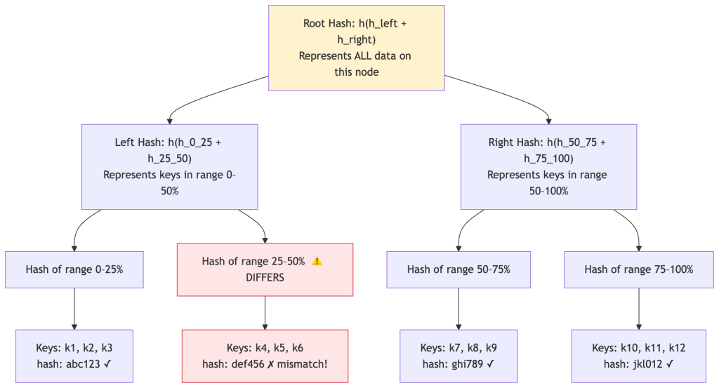
Leaf nodes contain the hash of a small range of actual data keys (e.g., hash of all values for keys k1, k2, k3).
Internal nodes contain the hash of their children’s hashes.
The root is a single hash representing all the data on the node.

How Two Nodes Sync Using Merkle Trees

When Node A and Node B want to check if they’re in sync:

Step 1: Compare root hashes. If they’re the same, everything is identical. Done! (No network traffic for the data itself.)

Step 2: If roots differ, compare their left children. Same? Skip that entire half of the key space.

Step 3: Keep descending only into subtrees where hashes differ, until you reach the leaf nodes.

Step 4: Sync only the specific keys in the differing leaf nodes.

			
Example: Comparing two nodes
Node A root: abc789  ← differs from Node B!
Node B root: abc788
Compare left subtrees:
  Node A left:  xyz123
  Node B left:  xyz123  ← same! Skip entire left half.
Compare right subtrees:
  Node A right: def456
  Node B right: def457  ← differs! Go deeper.
Compare right-left subtree:
  Node A right-left: ghi111
  Node B right-left: ghi111  ← same! Skip.
Compare right-right subtree:
  Node A right-right: jkl222
  Node B right-right: jkl333  ← differs! These are leaves.
→ Sync only the keys in the right-right leaf range (e.g., k10, k11, k12)
  Instead of comparing all 1 million keys, we compared 6 hashes
  and synced only 3 keys!

		

Synchronization process in code:

			
def sync_replicas(node_a, node_b, key_range):
    """
    Efficiently sync two nodes using Merkle trees.
    Instead of comparing all keys, we compare hashes top-down.
    Only the ranges where hashes differ need actual key-level sync.
    """
    tree_a = node_a.get_merkle_tree(key_range)
    tree_b = node_b.get_merkle_tree(key_range)
    # Step 1: Compare root hashes first.
    # If they match, every key in this range is identical — nothing to do!
    if tree_a.root_hash == tree_b.root_hash:
        return  # Zero data transferred — full match!
    # Step 2: Recursively find differences by traversing top-down.
    # Only descend into subtrees where hashes differ.
    differences = []
    stack = [(tree_a.root, tree_b.root)]
    while stack:
        node_a_subtree, node_b_subtree = stack.pop()
        if node_a_subtree.hash == node_b_subtree.hash:
            continue  # This whole subtree matches — skip it!
        if node_a_subtree.is_leaf:
            # Found a differing leaf — these keys need syncing
            differences.extend(node_a_subtree.keys)
        else:
            # Not a leaf yet — recurse into children
            for child_a, child_b in zip(node_a_subtree.children, node_b_subtree.children):
                stack.append((child_a, child_b))
    # Step 3: Sync only the specific keys that differed at leaf level.
    # This might be a handful of keys, not millions.
    for key in differences:
        sync_key(node_a, node_b, key)

		

Why This Is Efficient

The power of Merkle trees is that the number of hash comparisons you need scales with the depth of the tree (logarithmic in the number of keys), not the number of keys themselves.

			
Node with 1,000,000 keys:
Naive approach:  Compare 1,000,000 keys individually
                 Cost: 1,000,000 comparisons
Merkle tree:     Compare O(log N) hashes top-down
                 Tree depth ≈ 20 levels
                 Cost: 20 comparisons to find differences
                 Then sync only the differing leaves (~few keys)
Speedup: ~50,000x fewer comparisons!

		

And critically, if two nodes are mostly in sync (which is almost always true in a healthy cluster), the root hashes often match entirely and zero data needs to be transferred. The anti-entropy process is very cheap in the common case.

Membership and Failure Detection

Dynamo uses a gossip protocol for membership management. Each node periodically exchanges membership information with random peers. There is no master node—all coordination is fully decentralized.

Gossip-Based Membership

Key Design Points

No single coordinator: Every node maintains its own view of cluster membership. There’s no central registry, so there’s no single point of failure for membership data.

Failure suspicion vs. detection: Dynamo uses an accrual-based failure detector (similar to Phi Accrual). Rather than a binary “alive/dead” judgment, nodes maintain a suspicion level that rises the longer a peer is unresponsive. This avoids false positives from transient network hiccups.

			
Node A's view of Node B:
- Last heartbeat: 3 seconds ago → Suspicion low → Healthy
- Last heartbeat: 15 seconds ago → Suspicion rising → Likely slow/degraded
- Last heartbeat: 60 seconds ago → Suspicion high → Treat as failed

Decentralized bootstrapping: New nodes contact a seed node to join, then gossip spreads their presence to the rest of the cluster. Ring membership is eventually consistent—different nodes may have slightly different views of the ring momentarily, which is acceptable.

Performance Characteristics: Real Numbers

The paper provides fascinating performance data. Let me break it down:

Latency Distribution

			
Metric              | Average | 99.9th Percentile
--------------------|---------|------------------
Read latency        | ~10ms   | ~200ms
Write latency       | ~15ms   | ~200ms
Key insight: 99.9th percentile is ~20x the average!

		

Why the huge gap? The 99.9th percentile is affected by:

Garbage collection pauses
Disk I/O variations
Network jitter
Load imbalance

This is why Amazon SLAs are specified at 99.9th percentile, not average.

Version Conflicts

From 24 hours of Amazon’s production shopping cart traffic (per the Dynamo paper). Note these reflect Amazon’s specific workload characteristics, not a universal baseline:

			
94%    - Saw exactly one version (no conflict)
00057%  - Saw 2 versions
00047%  - Saw 3 versions  
00009%  - Saw 4 versions

Takeaway: Conflicts are rare in practice! Most often caused by concurrent writers (robots), not failures.

Partitioning Strategy Evolution

Dynamo evolved through three partitioning strategies. This evolution teaches us important lessons:

Strategy 1: Random Tokens (Initial)

			
Problem: Random token assignment → uneven load
Problem: Adding nodes → expensive data scans
Problem: Can't easily snapshot the system

Operational lesson: Random token assignment sounds elegant but is a nightmare in practice. Each node gets a random position on the ring, which means wildly different data ownership ranges and uneven load distribution.

Strategy 2: Equal-sized Partitions + Random Tokens

			
Improvement: Decouples partitioning from placement
Problem: Still has load balancing issues

Strategy 3: Q/S Tokens Per Node — Equal-sized Partitions + Deterministic Placement (Current)

What Q and S mean:

Q = the total number of fixed partitions the ring is divided into (e.g. 1024). Think of these as equally-sized, pre-cut slices of the hash space that never change shape.
S = the number of physical servers currently in the cluster (e.g. 8).
Q/S = how many of those fixed slices each server is responsible for (e.g. 1024 / 8 = 128 partitions per server).

The key shift from earlier strategies: the ring is now divided into Q fixed, equal-sized partitions first, and then those partitions are assigned evenly to servers. Servers no longer get random positions — they each own exactly Q/S partitions, distributed evenly around the ring.

			
Example: Q=12 partitions, S=3 servers
Ring divided into 12 equal slices (each covers 30° of the 360° ring):
  Partition  1:   0°– 30°  → Server A
  Partition  2:  30°– 60°  → Server B
  Partition  3:  60°– 90°  → Server C
  Partition  4:  90°–120°  → Server A
  Partition  5: 120°–150°  → Server B
  Partition  6: 150°–180°  → Server C
  ...and so on, round-robin
Each server owns exactly Q/S = 12/3 = 4 partitions → perfectly balanced.
When a 4th server joins (S becomes 4):
  New Q/S = 12/4 = 3 partitions per server.
  Each existing server hands off 1 partition to the new server.
  Only 3 out of 12 partitions move — the rest are untouched.

		

			
Benefits:
✓ Perfectly even load distribution (every server owns the same number of partitions)
✓ Fast bootstrapping — a joining node receives whole partition files, not scattered key ranges
✓ Easy archival — each partition is a self-contained file that can be snapshotted independently
✓ Membership metadata shrinks from multiple MB (hundreds of random tokens) to a few KB (a simple partition-to-server table)

		

This evolution — from random tokens to fixed, equal-sized partitions with balanced ownership — is one of the most instructive operational learnings from Dynamo. The early approach prioritized simplicity of implementation; the later approach prioritized operational simplicity and predictability.

Comparing Dynamo to Modern Systems

Let’s see how Dynamo concepts appear in systems you might use today:

System	Consistency Model	Use Case	Dynamo Influence
Cassandra	Tunable (N, R, W)	Time-series, analytics	Direct descendant — heavily inspired by Dynamo, uses same consistent hashing and quorum concepts
Riak	Tunable, vector clocks	Key-value store	Closest faithful Dynamo implementation
Amazon DynamoDB	Eventually consistent by default	Managed NoSQL	⚠️ Not the same as Dynamo! DynamoDB is a completely different system internally, with no vector clocks and much simpler conflict resolution. Shares the name and high-level inspiration only.
Voldemort	Tunable	LinkedIn’s data store	Open-source Dynamo implementation
Google Spanner	Linearizable	Global SQL	Opposite choice to Dynamo — prioritizes CP via TrueTime clock synchronization
Redis Cluster	Eventually consistent	Caching, sessions	Uses consistent hashing; much simpler conflict resolution

The DynamoDB confusion: Many engineers conflate Amazon DynamoDB with the Dynamo paper. They are very different. DynamoDB is a managed service optimized for operational simplicity. It does not expose vector clocks, does not use the same partitioning scheme, and uses a proprietary consistency model. The paper is about the internal Dynamo storage engine that predates DynamoDB.

What Dynamo Does NOT Give You

Every senior engineer blog should be honest about limitations. Here’s what Dynamo explicitly trades away:

No transactions: Operations are single-key only. You can’t atomically update multiple keys.
No secondary indexes: You can only look up data by its primary key (at least in the original design).
No joins: It’s a key-value store. There is no query language.
No global ordering: Events across different keys have no guaranteed ordering.
No linearizability: Even at R=W=N, Dynamo does not provide linearizable reads. There is no global clock, no strict serializability.
No automatic conflict resolution: The system detects conflicts and surfaces them to the application. The application must resolve them. If your engineers don’t understand this, you will have subtle data bugs.
Repair costs at scale: The anti-entropy process (Merkle tree reconciliation) is not free. At large scale, background repair traffic can be significant.
Vector clock growth: In high-churn write environments with many coordinators, vector clocks can grow large enough to require truncation, which introduces potential causality loss.

Understanding these limitations is critical to successfully operating Dynamo-style systems in production.

Practical Implementation Example

Below is a self-contained Python implementation of the core Dynamo concepts. It’s intentionally simplified—no actual networking, no persistence—but it faithfully models how vector clocks, the consistent hash ring, quorum reads/writes, and conflict detection interact. Each component is explained before its code.

Part 1: Vector Clock

The VectorClock class is the foundation of version tracking. It’s just a dictionary mapping node_id → counter. Two key operations:

increment(node) — bump our own counter when we write
dominates(other) — check if one clock is causally “after” another; if neither dominates, the writes were concurrent (conflict)

			
from __future__ import annotations
from dataclasses import dataclass, field
from typing import Optional
class VectorClock:
    """
    Tracks causality across distributed writes.
    A clock like {"nodeA": 2, "nodeB": 1} means:
      - nodeA has coordinated 2 writes
      - nodeB has coordinated 1 write
      - Any version with these counters has "seen" those writes
    """
    def __init__(self, clock: dict[str, int] | None = None):
        self.clock: dict[str, int] = clock.copy() if clock else {}
    def increment(self, node_id: str) -> "VectorClock":
        """Return a new clock with node_id's counter bumped by 1."""
        new_clock = self.clock.copy()
        new_clock[node_id] = new_clock.get(node_id, 0) + 1
        return VectorClock(new_clock)
    def dominates(self, other: "VectorClock") -> bool:
        """
        Returns True if self is causally AFTER other.
        self dominates other when:
          - Every counter in self is >= the same counter in other, AND
          - At least one counter in self is strictly greater.
        Meaning: self has seen everything other has seen, plus more.
        """
        all_keys = set(self.clock) | set(other.clock)
        at_least_one_greater = False
        for key in all_keys:
            self_val = self.clock.get(key, 0)
            other_val = other.clock.get(key, 0)
            if self_val < other_val:
                return False  # self is missing something other has seen
            if self_val > other_val:
                at_least_one_greater = True
        return at_least_one_greater
    def merge(self, other: "VectorClock") -> "VectorClock":
        """
        Merge two clocks by taking the max of each counter.
        Used after resolving a conflict to produce a new clock
        that has "seen" everything both conflicting versions saw.
        """
        all_keys = set(self.clock) | set(other.clock)
        merged = {k: max(self.clock.get(k, 0), other.clock.get(k, 0)) for k in all_keys}
        return VectorClock(merged)
    def __repr__(self):
        return f"VectorClock({self.clock})"

		

Part 2: Versioned Value

Every value stored in Dynamo is wrapped with its vector clock. This pairing is what allows the coordinator to compare versions during reads and detect conflicts.

			
@dataclass
class VersionedValue:
    """
    A value paired with its causal history (vector clock).
    When a client reads, they get back a VersionedValue.
    When they write an update, they must include the context
    (the vector clock they read) so Dynamo knows what version
    they're building on top of.
    """
    value: object
    vector_clock: VectorClock
    def __repr__(self):
        return f"VersionedValue(value={self.value!r}, clock={self.vector_clock})"

		

Part 3: Simulated Node

In real Dynamo each node is a separate process. Here we simulate them as in-memory objects. The key detail: each node has its own local storage dict. Nodes can be marked as down to simulate failures.

			
class DynamoNode:
    """
    Simulates a single Dynamo storage node.
    In production this would be a separate server with disk storage.
    Here it's an in-memory dict so we can demo the logic without networking.
    """
    def __init__(self, node_id: str, token: int):
        self.node_id = node_id
        self.token = token          # Position on the consistent hash ring
        self.storage: dict[str, list[VersionedValue]] = {}
        self.down = False           # Toggle to simulate node failures
    def write(self, key: str, versioned_value: VersionedValue) -> bool:
        """
        Store a versioned value. Returns False if the node is down.
        We store a LIST of versions per key, because a node might
        hold multiple concurrent (conflicting) versions until they
        are resolved by the application.
        """
        if self.down:
            return False
        # In a real node this would be written to disk (e.g. BerkeleyDB)
        self.storage[key] = [versioned_value]
        return True
    def read(self, key: str) -> list[VersionedValue] | None:
        """
        Return all versions of a key. Returns None if the node is down.
        A healthy node with no data for the key returns an empty list.
        """
        if self.down:
            return None
        return self.storage.get(key, [])
    def __repr__(self):
        status = "DOWN" if self.down else f"token={self.token}"
        return f"DynamoNode({self.node_id}, {status})"

		

Part 4: Consistent Hash Ring

The ring maps keys to nodes. We sort nodes by their token (position) and use a clockwise walk to find the coordinator and preference list for any key.

			
import hashlib
class ConsistentHashRing:
    """
    Maps any key to an ordered list of N nodes (the preference list).
    Nodes are placed at fixed positions (tokens) on a conceptual ring
    from 0 to 2^32. A key hashes to a position, then walks clockwise
    to find its nodes.
    This means adding/removing one node only rebalances ~1/N of keys,
    rather than reshuffling everything like modulo hashing would.
    """
    def __init__(self, nodes: list[DynamoNode]):
        # Sort nodes by token so we can do clockwise lookup efficiently
        self.nodes = sorted(nodes, key=lambda n: n.token)
    def _hash(self, key: str) -> int:
        """Consistent hash of a key into the ring's token space."""
        # Use MD5 for a simple, evenly distributed hash.
        # Real Dynamo uses a more sophisticated hash (e.g., SHA-1).
        digest = hashlib.md5(key.encode()).hexdigest()
        return int(digest, 16) % (2**32)
    def get_preference_list(self, key: str, n: int) -> list[DynamoNode]:
        """
        Return the first N nodes clockwise from key's hash position.
        These are the nodes responsible for storing this key.
        The first node in the list is the coordinator — it receives
        the client request and fans out to the others.
        """
        if not self.nodes:
            return []
        key_hash = self._hash(key)
        # Find the first node whose token is >= key's hash (clockwise)
        start_idx = 0
        for i, node in enumerate(self.nodes):
            if node.token >= key_hash:
                start_idx = i
                break
            # If key_hash is greater than all tokens, wrap around to node 0
            else:
                start_idx = 0
        # Walk clockwise, collecting N unique nodes
        preference_list = []
        for i in range(len(self.nodes)):
            idx = (start_idx + i) % len(self.nodes)
            preference_list.append(self.nodes[idx])
            if len(preference_list) == n:
                break
        return preference_list

		

Part 5: The Dynamo Coordinator

This is the heart of the system — the logic that handles client requests, fans out to replicas, waits for quorum, and detects conflicts. Study this carefully; it’s where all the earlier concepts converge.

			
class SimplifiedDynamo:
    """
    Coordinates reads and writes across a cluster of DynamoNodes.
    Any node can act as coordinator for any request — there's no
    dedicated master. The coordinator is simply whichever node
    receives the client request (or the first node in the preference
    list, if using partition-aware routing).
    Configuration:
      N = total replicas per key
      R = minimum nodes that must respond to a read (read quorum)
      W = minimum nodes that must acknowledge a write (write quorum)
    """
    def __init__(self, nodes: list[DynamoNode], N: int = 3, R: int = 2, W: int = 2):
        self.N = N
        self.R = R
        self.W = W
        self.ring = ConsistentHashRing(nodes)
    # ------------------------------------------------------------------ #
    #  WRITE                                                               #
    # ------------------------------------------------------------------ #
    def put(self, key: str, value: object,
            context: VectorClock | None = None) -> VectorClock:
        """
        Write a key-value pair to N replicas, wait for W ACKs.
        The 'context' is the vector clock from a previous read.
        Always pass context when updating an existing key — it tells
        Dynamo which version you're building on top of, so it can
        detect whether your write is concurrent with anything else.
        Returns the new vector clock, which the caller should store
        and pass back on future writes to this key.
        Raises: RuntimeError if fewer than W nodes acknowledged.
        """
        preference_list = self.ring.get_preference_list(key, self.N)
        if not preference_list:
            raise RuntimeError("No nodes available")
        # The coordinator is always the first node in the preference list.
        coordinator = preference_list[0]
        # Increment the coordinator's counter in the vector clock.
        # If no context was provided (brand new key), start a fresh clock.
        base_clock = context if context is not None else VectorClock()
        new_clock = base_clock.increment(coordinator.node_id)
        versioned = VersionedValue(value=value, vector_clock=new_clock)
        # Fan out to all N replicas.
        # In a real system these would be concurrent RPC calls.
        # Here we call them sequentially for simplicity.
        ack_count = 0
        for node in preference_list:
            success = node.write(key, versioned)
            if success:
                ack_count += 1
        # Only need W ACKs to declare success.
        # The remaining replicas are updated asynchronously (or via
        # hinted handoff if they were down).
        if ack_count < self.W:
            raise RuntimeError(
                f"Write quorum not met: got {ack_count} ACKs, needed {self.W}"
            )
        print(f"[PUT] key={key!r}  value={value!r}  clock={new_clock}  "
              f"({ack_count}/{self.N} nodes wrote)")
        return new_clock
    # ------------------------------------------------------------------ #
    #  READ                                                                #
    # ------------------------------------------------------------------ #
    def get(self, key: str) -> list[VersionedValue]:
        """
        Read a key from N replicas, wait for R responses, reconcile.
        Returns a LIST of VersionedValues:
          - Length 1  → clean read, no conflict
          - Length >1 → concurrent versions detected; application must merge
        After reading, the caller should:
          1. If no conflict: use the single value normally.
          2. If conflict: merge the values using application logic,
             then call put() with the merged value and the merged
             vector clock as context. This "closes" the conflict.
        Read repair happens in the background: any replica that returned
        a stale version is silently updated with the latest version.
        """
        preference_list = self.ring.get_preference_list(key, self.N)
        # Collect responses from all N nodes
        all_versions: list[VersionedValue] = []
        responding_nodes: list[tuple[DynamoNode, list[VersionedValue]]] = []
        for node in preference_list:
            result = node.read(key)
            if result is not None:   # None means the node is down
                all_versions.extend(result)
                responding_nodes.append((node, result))
        if len(responding_nodes) < self.R:
            raise RuntimeError(
                f"Read quorum not met: got {len(responding_nodes)} responses, needed {self.R}"
            )
        # Reconcile: discard any version that is strictly dominated
        # (i.e., is a causal ancestor of) another version.
        # What remains is the set of concurrent versions.
        reconciled = self._reconcile(all_versions)
        # Background read repair: if any node returned something older
        # than the reconciled result, send it the latest version.
        # (Simplified: only meaningful when there's a single winner.)
        if len(reconciled) == 1:
            latest = reconciled[0]
            for node, versions in responding_nodes:
                if not versions or versions[0].vector_clock != latest.vector_clock:
                    node.write(key, latest)   # Repair silently in background
        status = "clean" if len(reconciled) == 1 else f"CONFLICT ({len(reconciled)} versions)"
        print(f"[GET] key={key!r}  status={status}  "
              f"({len(responding_nodes)}/{self.N} nodes responded)")
        return reconciled
    # ------------------------------------------------------------------ #
    #  INTERNAL: VERSION RECONCILIATION                                   #
    # ------------------------------------------------------------------ #
    def _reconcile(self, versions: list[VersionedValue]) -> list[VersionedValue]:
        """
        Remove any version that is a causal ancestor of another version.
        If version A's clock is dominated by version B's clock, then B
        is strictly newer — A adds no new information and can be dropped.
        Whatever remains after pruning are CONCURRENT versions: writes
        that happened without either "knowing about" the other.
        The application must merge these using domain-specific logic.
        Example:
          versions = [clock={A:1}, clock={A:2}, clock={B:1}]
          {A:2} dominates {A:1}  → drop {A:1}
          {A:2} and {B:1} are concurrent → both survive
          result = [{A:2}, {B:1}]  ← conflict! application must merge
        """
        dominated = set()
        for i, v1 in enumerate(versions):
            for j, v2 in enumerate(versions):
                if i != j and v2.vector_clock.dominates(v1.vector_clock):
                    dominated.add(i)   # v1 is an ancestor of v2, discard v1
        survivors = [v for i, v in enumerate(versions) if i not in dominated]
        # De-duplicate: identical clocks from different replicas are the same version
        seen_clocks: list[VectorClock] = []
        unique: list[VersionedValue] = []
        for v in survivors:
            if not any(v.vector_clock.clock == s.clock for s in seen_clocks):
                unique.append(v)
                seen_clocks.append(v.vector_clock)
        return unique if unique else versions

		

Part 6: Putting It All Together — A Demo

Let’s run through a complete scenario: normal write/read, then a simulated conflict where two nodes diverge and the application must merge them.

			
def demo():
    # ── Setup ────────────────────────────────────────────────────────── #
    # Five nodes placed at evenly spaced positions on the hash ring.
    # In a real cluster these would span multiple datacenters.
    nodes = [
        DynamoNode("node-A", token=100),
        DynamoNode("node-B", token=300),
        DynamoNode("node-C", token=500),
        DynamoNode("node-D", token=700),
        DynamoNode("node-E", token=900),
    ]
    dynamo = SimplifiedDynamo(nodes, N=3, R=2, W=2)
    print("=" * 55)
    print("SCENARIO 1: Normal write and read (no conflict)")
    print("=" * 55)
    # Write the initial shopping cart
    ctx = dynamo.put("cart:user-42", {"items": ["shoes"]})
    # Read it back — should be a clean single version
    versions = dynamo.get("cart:user-42")
    print(f"Read result: {versions[0].value}\n")
    # Update the cart, passing the context from our earlier read.
    # The context tells Dynamo "this write builds on top of clock ctx".
    ctx = dynamo.put("cart:user-42", {"items": ["shoes", "jacket"]}, context=ctx)
    versions = dynamo.get("cart:user-42")
    print(f"After update: {versions[0].value}\n")
    print("=" * 55)
    print("SCENARIO 2: Simulated conflict — two concurrent writes")
    print("=" * 55)
    # Write the base version
    base_ctx = dynamo.put("cart:user-99", {"items": ["hat"]})
    # Now simulate a network partition:
    # node-A and node-B can't talk to each other.
    # We model this by writing directly to individual nodes.
    pref_list = dynamo.ring.get_preference_list("cart:user-99", 3)
    node_1, node_2, node_3 = pref_list[0], pref_list[1], pref_list[2]
    # Write 1: customer adds "scarf" via node_1 (e.g., their laptop)
    clock_1 = base_ctx.increment(node_1.node_id)
    node_1.write("cart:user-99", VersionedValue({"items": ["hat", "scarf"]}, clock_1))
    # Write 2: customer adds "gloves" via node_2 (e.g., their phone)
    # This write also descends from base_ctx, not from clock_1.
    # Neither write knows about the other → they are concurrent.
    clock_2 = base_ctx.increment(node_2.node_id)
    node_2.write("cart:user-99", VersionedValue({"items": ["hat", "gloves"]}, clock_2))
    # Read — coordinator sees two concurrent versions and surfaces the conflict
    versions = dynamo.get("cart:user-99")
    if len(versions) > 1:
        print(f"\nConflict detected! {len(versions)} concurrent versions:")
        for i, v in enumerate(versions):
            print(f"  Version {i+1}: {v.value}  clock={v.vector_clock}")
        # Application-level resolution: union merge (Amazon's shopping cart strategy)
        # Merge items: take the union so no addition is lost
        all_items = set()
        merged_clock = versions[0].vector_clock
        for v in versions:
            all_items.update(v.value["items"])
            merged_clock = merged_clock.merge(v.vector_clock)
        merged_value = {"items": sorted(all_items)}
        print(f"\nMerged result: {merged_value}")
        # Write the resolved version back with the merged clock as context.
        # This "closes" the conflict — future reads will see a single version.
        final_ctx = dynamo.put("cart:user-99", merged_value, context=merged_clock)
        versions = dynamo.get("cart:user-99")
        print(f"\nAfter resolution: {versions[0].value}")
        assert len(versions) == 1, "Should be a single version after merge"
if __name__ == "__main__":
    demo()

		

Expected output:

			
=======================================================
SCENARIO 1: Normal write and read (no conflict)
=======================================================
[PUT] key='cart:user-42'  value={'items': ['shoes']}  clock=VectorClock({'node-A': 1})  (3/3 nodes wrote)
[GET] key='cart:user-42'  status=clean  (3/3 nodes responded)
Read result: {'items': ['shoes']}
[PUT] key='cart:user-42'  value={'items': ['shoes', 'jacket']}  clock=VectorClock({'node-A': 2})  (3/3 nodes wrote)
[GET] key='cart:user-42'  status=clean  (3/3 nodes responded)
After update: {'items': ['shoes', 'jacket']}
=======================================================
SCENARIO 2: Simulated conflict — two concurrent writes
=======================================================
[PUT] key='cart:user-99'  value={'items': ['hat']}  clock=VectorClock({'node-A': 1})  (3/3 nodes wrote)
[GET] key='cart:user-99'  status=CONFLICT (2 versions)  (3/3 nodes responded)
Conflict detected! 2 concurrent versions:
  Version 1: {'items': ['hat', 'scarf']}  clock=VectorClock({'node-A': 2})
  Version 2: {'items': ['hat', 'gloves']}  clock=VectorClock({'node-A': 1, 'node-B': 1})
Merged result: {'items': ['gloves', 'hat', 'scarf']}
[PUT] key='cart:user-99'  value={'items': ['gloves', 'hat', 'scarf']}  ...  (3/3 nodes wrote)
[GET] key='cart:user-99'  status=clean  (3/3 nodes responded)
After resolution: {'items': ['gloves', 'hat', 'scarf']}

		

What to notice: In Scenario 2, the coordinator correctly identifies that {'node-A': 2} and {'node-A': 1, 'node-B': 1} are neither equal nor in a dominance relationship — neither is an ancestor of the other — so both are surfaced as concurrent. The application then takes responsibility for merging them and writing back a resolved version with the merged clock.

Key Lessons for System Design

After working with Dynamo-inspired systems for years, here are my key takeaways:

1. Always-On Beats Strongly-Consistent

For user-facing applications, availability almost always wins. Users will tolerate seeing slightly stale data. They won’t tolerate “Service Unavailable.”

2. Application-Level Reconciliation is Powerful

Don’t be afraid to push conflict resolution to the application. The application understands the business logic and can make smarter decisions than the database ever could.

3. Tunable Consistency is Essential

One size doesn’t fit all. Shopping cart additions need high availability (W=1). Financial transactions need stronger guarantees (W=N). The ability to tune this per-operation is incredibly valuable.

4. The 99.9th Percentile Matters More Than Average

Focus your optimization efforts on tail latencies. That’s what users actually experience during peak times.

5. Gossip Protocols Scale Beautifully

Decentralized coordination via gossip eliminates single points of failure and scales to thousands of nodes.

When NOT to Use Dynamo-Style Systems

Be honest about trade-offs. Don’t use this approach when:

Strong consistency is required (financial transactions, inventory management)
Complex queries are needed (reporting, analytics, joins)
Transactions span multiple items (Dynamo is single-key operations only)
Your team can’t handle eventual consistency (if developers don’t understand vector clocks and conflict resolution, you’ll have problems)

Conclusion

Dynamo represents a fundamental shift in how we think about distributed systems. By embracing eventual consistency and providing tunable trade-offs, it enables building systems that scale to massive sizes while maintaining high availability.

The paper’s lessons have influenced an entire generation of distributed databases. Whether you’re using Cassandra, Riak, or DynamoDB, you’re benefiting from the insights first published in this paper.

As engineers, our job is to understand these trade-offs deeply and apply them appropriately. Dynamo gives us a powerful tool, but like any tool, it’s only as good as our understanding of when and how to use it.

Appendix: Design Problems and Approaches

Three open-ended problems that come up in system design interviews and real engineering work. Think through each before reading the discussion.

Problem 1: Conflict Resolution for a Collaborative Document Editor

The problem: You’re building something like Google Docs backed by a Dynamo-style store. Two users edit the same paragraph simultaneously. How do you handle the conflict?

Why shopping cart union doesn’t work here: The shopping cart strategy (union of all items) is only safe because adding items is commutative — {A} ∪ {B} = {B} ∪ {A}. Text editing is not commutative. If User A deletes a sentence and User B edits the middle of it, the union of their changes is meaningless or contradictory.

The right approach: Operational Transformation (OT) or CRDTs

The industry solution is to represent the document not as a blob of text, but as a sequence of operations, and to transform concurrent operations so they can both be applied without conflict:

			
User A's operation: delete(position=50, length=20)
User B's operation: insert(position=60, text="new sentence")
Without OT: B's insert position (60) is now wrong because A deleted 20 chars.
With OT:    Transform B's operation against A's:
            B's insert position shifts to 40 (60 - 20).
            Both operations now apply cleanly.

		

The conflict resolution strategy for the Dynamo layer would be:

Store operations (not full document snapshots) as the value for each key.
On conflict, collect all concurrent operation lists from each version.
Apply OT to merge them into a single consistent operation log.
Write the merged log back with the merged vector clock as context.

What to store in Dynamo: The operation log per document segment, not the rendered text. This makes merges deterministic and lossless.

Real-world reference: This is essentially how Google Docs, Notion, and Figma work. Their storage layers use either OT or a variant of CRDTs (Conflict-free Replicated Data Types), which are data structures mathematically guaranteed to merge without conflicts regardless of operation ordering.

Problem 2: Choosing N, R, W for Different Use Cases

The problem: What configuration would you pick for (a) a session store, (b) a product catalog, (c) user profiles?

The right way to think about this: identify the failure mode that costs more — a missed write (data loss) or a rejected write (unavailability). Then pick quorum values accordingly.

Session store — prioritize availability

Sessions are temporary and user-specific. If a user’s session is briefly stale or lost, they get logged out and log back in. That’s annoying but not catastrophic. You never want to reject a session write.

			
N=3, R=1, W=1
Rationale:
- W=1: Accept session writes even during heavy failures.
        A user can't log in if their session write is rejected.
- R=1: Read from any single node. Stale session data is harmless.
- N=3: Still replicate to 3 nodes for basic durability.
Trade-off accepted: Stale session reads are possible but inconsequential.

		

Product catalog — prioritize read performance and consistency

Product data is written rarely (by ops teams) but read millions of times per day. Stale prices or descriptions are problematic. You want fast, consistent reads.

			
N=3, R=2, W=3
Rationale:
- W=3: All replicas must confirm a catalog update before it's live.
        A price change half-published is worse than a brief write delay.
- R=2: Read quorum overlap with W=3 guarantees fresh data.
        Acceptable: catalog writes are rare, so write latency doesn't matter.
- N=3: Standard replication for durability.
Trade-off accepted: Writes are slow and fail if any node is down.
                    Acceptable because catalog updates are infrequent.

		

User profiles — balanced

Profile data (name, email, preferences) is moderately important. A stale profile is annoying but not dangerous. A rejected update (e.g., user can’t update their email) is a real problem.

			
N=3, R=2, W=2
Rationale:
- The classic balanced configuration.
- R + W = 4 > N = 3, so quorums overlap: reads will see the latest write.
- Tolerates 1 node failure for both reads and writes.
- Appropriate for data that matters but doesn't require strict consistency.
Trade-off accepted: A second simultaneous node failure will cause errors.
                    Acceptable for non-critical user data.

		

Decision framework summary:

Priority	R	W	When to use
Max availability	1	1	Sessions, ephemeral state, click tracking
Balanced	2	2	User profiles, preferences, soft state
Consistent reads	2	3	Catalogs, config, rarely-written reference data
Highest consistency	3	3	Anywhere you need R+W > N with zero tolerance for stale reads (still not linearizable)

Problem 3: Testing a Dynamo-Style System Under Partition Scenarios

The problem: How do you verify that your system actually behaves correctly when nodes fail and partitions occur?

This is one of the hardest problems in distributed systems testing because the bugs only appear in specific interleavings of concurrent events that are difficult to reproduce deterministically.

Layer 1: Unit tests for the logic in isolation

Before testing distributed behavior, verify the building blocks independently. Vector clock comparison logic, conflict detection, and reconciliation functions can all be tested with pure unit tests — no networking needed.

			
def test_concurrent_clocks_detected_as_conflict():
    clock_a = VectorClock({"node-A": 2})
    clock_b = VectorClock({"node-B": 2})
    assert not clock_a.dominates(clock_b)
    assert not clock_b.dominates(clock_a)
    # Both survive reconciliation → conflict correctly detected
def test_ancestor_clock_is_discarded():
    old_clock = VectorClock({"node-A": 1})
    new_clock = VectorClock({"node-A": 3})
    assert new_clock.dominates(old_clock)
    # old_clock should be pruned during reconciliation

		

Layer 2: Deterministic fault injection

Rather than hoping failures happen in the right order during load testing, inject them deliberately and repeatably. In the demo implementation above, node.down = True is a simple version of this. In production systems, libraries like Jepsen or Chaos Monkey do this at the infrastructure level.

Key scenarios to test:

			
Scenario A: Write succeeds with W=2, third replica is down.
  → Verify: the data is readable after the down node recovers.
  → Verify: no data loss occurred.
Scenario B: Two nodes accept concurrent writes to the same key.
  → Verify: the next read surfaces exactly 2 conflicting versions.
  → Verify: after the application writes a merged version, the next read is clean.
Scenario C: Node goes down mid-write (wrote to W-1 nodes).
  → Verify: the write is correctly rejected (RuntimeError).
  → Verify: no partial writes are visible to readers.
Scenario D: All N nodes recover after a full partition.
  → Verify: no data was lost across the cluster.
  → Verify: vector clocks are still meaningful (no spurious conflicts).

		

Layer 3: Property-based testing

Instead of writing individual test cases, define invariants that must always hold and generate thousands of random operation sequences to try to violate them:

			
# Invariant: after any sequence of writes and merges, a final get()
# should always return exactly one version (no unresolved conflicts).
# Invariant: a value written with a context derived from a previous read
# should never produce a conflict with that read's version
# (it should dominate it).
# Invariant: if R + W > N, a value written successfully should always
# be visible in the next read (read-your-writes, absent concurrent writes).

		

Tools like Hypothesis (Python) let you express these invariants and automatically find counterexamples.

Layer 4: Linearizability checkers

For the highest confidence, record every operation’s start time, end time, and result during a fault injection test, then feed the history to a linearizability checker like Knossos. It will tell you whether any observed history is consistent with a correct sequential execution — even for an eventually-consistent system operating within its stated guarantees.

Written from the trenches of distributed systems. Battle-tested insights, zero hand-waving.

NotebookLM Link